Chapter 3. Dynamics

R C

R1

I

V

−

V1

V2

Figure 3.6 Schematic diagram of an electric circuit.

EXAMPLE 3.5—OPERATIONAL AMPLIFIERS

Consider the electric circuit shown in Figure 3.6. Assume that the problem is to find the relation between the input voltage V1 and the output voltage V2. Assuming that the gain of the amplifier is very high, say around 106, then the voltage V is negligible and the current I0 is zero. The currents I1 and I2 then are the same which gives

LV1 − LV2

Z1DsE Z2DsE

It now remains to determine the generalized impedances Z1 and Z2. The impedance Z2 is a regular resistor. To determine Z1 we use the simple rule for combining resistors which gives

Z1DsE R

1

sC

Hence

Z1DsE

LV2

−

−

R

−

1

LV2

Z2DsE

R2

R2 Cs

Converting to the time domain we find

R

1

Z0

t

V2DtE −

V1Dτ Edτ

−

R2

R2 C

The circuit is thus a PI controller.

3.5 Frequency Response

The idea of frequency response is to characterize linear time-invariant systems by their response to sinusoidal signals. The idea goes back to

90

3.5 Frequency Response

		0.2
		0.15
Output		0.1
		0.05
		0
	−0.05
		−0.1	5	10	15
		0
		1
		0.5
Input		0
		−0.5
		−1	5	10	15
		0
				Time

Figure 3.7 Response of a linear time-invariant system to a sinusoidal input Dfull linesE. The dashed line shows the steady state output calculated from D3.23E.

Fourier, who introduced the method to investigate propagation of heat in metals. Figure 3.7 shows the response of a linear time-invariant system to a sinusoidal input. The figure indicates that after a transient the output is a sinusoid with the same frequency as the input. The steady state response to a sinusoidal input of a stable linear system is in fact given by GDiω E. Hence if the input is

uDtE a sin ω t a eiω t

the output is

yDtE ahGDiω Eh sin Dω t arg GDiω EE a eiω t GDiω E

D3.23E

The dashed line in Figure 3.7 shows the output calculated by this formula. It follows from this equation that the transfer function G has the interesting property that its value for s iω describes the steady state response to sinusoidal signals. The function GDiω E is therefore called the frequency response. The argument of the function is frequency ω and the function takes complex values. The magnitude gives the magnitude of the steady state output for a unit amplitude sinusoidal input and the argument gives the phase shift between the input and the output. Notice that the system must be stable for the steady state output to exist.

91

Chapter 3. Dynamics

The frequency response can be determined experimentally by analyzing how a system responds to sinusoidal signals. It is possible to make very accurate measurements by using correlation techniques.

To derive the formula we will first calculate the response of a system with the transfer function GDsE to the signal eat where all poles of the transfer function have the property pk α a. The Laplace transform

of the output is

YDsE GDsEs −1 a

Making a partial fraction expansion we get

	Y s		GDaE		Rk
		E s − a		X Ds − pkEDpk − aE
	D

It follows the output has the property

yDtE − GDaEeat ce−α t

where c is a constant. Asymptotically we thus find that the output approaches GDaEeat. Setting a ib we find that the response to the input

uDtE eibt cos bt i sin bt

will approach

yDtE GDibEeibt hGDibEheiDb arg GDibEE

hGDibEh cos Dbt arg arg GDibEE ihGDibEh sin Dbt arg arg GDibEE

Separation of real and imaginary parts give the result.

Nyquist Plots

The response of a system to sinusoids is given by the the frequency response GDiω E. This function can be represented graphically by plotting the magnitude and phase of GDiω E for all frequencies, see Figure 3.8. The magnitude a hGDiω Eh represents the amplitude of the output and the angle φ arg GDiω E represents the phase shift. The phase shift is typically negative which implies that the output will lag the input. The angle ψ in the figure is therefore called phase lag. One reason why the Nyquist curve is important is that it gives a totally new way of looking at stability of a feedback system. Consider the feedback system in Figure 3.9. To investigate stability of a the system we have to derive the characteristic equation of the closed loop system and determine if all its roots are in the left half plane. Even if it easy to determine the roots of the equation

92

3.5 Frequency Response

			Im G(iω)
Ultimate point
				Re G(iω)
−		1	ϕ
				a
				ω

Figure 3.8 The Nyquist plot of a transfer function GDiw E.

B	A
	LDsE
	−1

Figure 3.9 Block diagram of a simple feedback system.

numerically it is not easy to determine how the roots are influenced by the properties of the controller. It is for example not easy to see how to modify the controller if the closed loop system is stable. We have also defined stability as a binary property, a system is either stable or unstable. In practice it is useful to be able to talk about degrees of stability. All of these issues are addressed by Nyquist's stability criterion. This result has a strong intuitive component which we will discuss first. There is also some beautiful mathematics associated with it that will be discussed in a separate section.

Consider the feedback system in Figure 3.9. Let the transfer functions of the process and the controller be PDsE and CDsE respectively. Introduce the loop transfer function

LDsE PDsECDsE

D3.24E

To get insight into the problem of stability we will start by investigating

93

Chapter 3. Dynamics

the conditions for oscillation. For that purpose we cut the feedback loop as indicated in the figure and we inject a sinusoid at point A. In steady state the signal at point B will also be a sinusoid with the same frequency. It seems reasonable that an oscillation can be maintained if the signal at B has the same amplitude and phase as the injected signal because we could then connect A to B. Tracing signals around the loop we find that the condition that the signal at B is identical to the signal at A is that

LDiω 0E −1

D3.25E

which we call the condition for oscillation. This condition means that the Nyquist curve of LDiω E intersects the negative real axis at the point -1. Intuitively it seems reasonable that the system would be stable if the Nyquist curve intersects to the right of the point -1 as indicated in Figure 3.9. This is essentially true, but there are several subtleties that are revealed by the proper theory.

Stability Margins

In practice it is not enough to require that the system is stable. There must also be some margins of stability. There are many ways to express this. Many of the criteria are based on Nyquist's stability criterion. They are based on the fact that it is easy to see the effects of changes of the gain and the phase of the controller in the Nyquist diagram of the loop transfer function LDsE. An increase of controller gain simply expands the Nyquist curve radially. An increase of the phase of the controller twists the Nyquist curve clockwise, see Figure 3.10. The gain margin nm tells how much the controller gain can be increased before reaching the stability limit. Let ω 180 be the smallest frequency where the phase lag of the loop transfer function LDsE is 180'. The gain margin is defined as

nm	1	D3.26E
	hLDiω 180Eh

The stability margin is a closely related concept which is defined as

1
sm 1 hLDiω 180Eh 1 −		D3.27E
	nm

A nice feature of the stability margin is that it is a number between 0 and 1. Values close to zero imply a small margin.

The phase margin ϕm is the amount of phase lag required to reach the stability limit. Let ω nc denote the lowest frequency where the loop transfer function LDsE has unit magnitude. The phase margin is then given by

ϕm π arg LDiω ncE

D3.28E

94

3.5 Frequency Response

Figure 3.10 Nyquist curve of the loop transfer function L with indication of gain, phase and stability margins.

The margins have simple geometric interpretations in the Nyquist diagram of the loop transfer function as is shown in Figure 3.10. The stability margin sm is the distance between the critical point and the intersection of the Nyquist curve with the negative real axis.

One possibility to characterize the stability margin with a single number is to choose the shortest distance d to the critical point. This is also shown in Figure 3.10.

Reasonable values of the margins are phase margin ϕm 30' − 60', gain margin nm 2 − 5, stability margin sm 0.5 − 0.8, and shortest distance to the critical point d 0.5 − 0.8.

The gain and phase margins were originally conceived for the case when the Nyquist curve only intersects the unit circle and the negative real axis once. For more complicated systems there may be many intersections and it is then necessary to consider the intersections that are closest to the critical point. For more complicated systems there is also another number that is highly relevant namely the delay margin. The delay margin is defined as the smallest time delay required to make the system unstable. For loop transfer functions that decay quickly the delay margin is closely related to the phase margin but for systems where the amplitude ratio of the loop transfer function has several peaks at high frequencies the delay margin is a much more relevant measure.

95

Chapter 3. Dynamics

Nyquist's Stability Theorem*

We will now prove the Nyquist stability theorem. This will require more results from the theory of complex variables than in many other parts of the book. Since precision is needed we will also use a more mathematical style of presentation. We will start by proving a key theorem about functions of complex variables.

THEOREM 3.1—PRINCIPLE OF VARIATION OF THE ARGUMENT

Let D be a closed region in the complex plane and let Γ be the boundary of the region. Assume the function f is analytic in D and on Γ except at a finite number of poles and zeros, then

wn 2π	Γ arg f DzE 2π i ZΓ		fPDDzEEdz N − P
1	1		f z

where N is the number of zeros and P the number of poles in D. Poles and zeros of multiplicity m are counted m times. The number wn is called the winding number and Γ arg f DzE is the variation of the argument of the function f as the curve Γ is traversed in the positive direction.

PROOF 3.1

Assume that z a is a zero of multiplicity m. In the neighborhood of

z a we have

f DzE Dz − aEmnDzE

where the function n is analytic and different form zero. We have

f PDzE		m		nPDzE
f DzE		z − a		nDzE

The second term is analytic at z a. The function f P/f thus has a single pole at z a with the residue m. The sum of the residues at the zeros of the function is N. Similarly we find that the sum of the residues of the poles of is −P. Furthermore we have

			d		log f		z		f PDzE
		dz							f DzE
							D E
which implies that	ZΓ		ffPDDzEEdz					Γ log f DzE
					z

where Γ denotes the variation along the contour Γ. We have log f DzE log hf DzEh i arg f DzE

96

3.5 Frequency Response

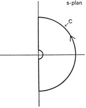
Figure 3.11 Contour Γ used to prove Nyquist's stability theorem.

Since the variation of hf DzEh around a closed contour is zero we have

Γ log f DzE i Γ arg f DzE

and the theorem is proven.

REMARK 3.1

The number wn is called the winding number.

REMARK 3.2

The theorem is useful to determine the number of poles and zeros of an function of complex variables in a given region. To use the result we must determine the winding number. One way to do this is to investigate how the curve Γ is transformed under the map f . The variation of the argument is the number of times the map of Γ winds around the origin in the f -plane. This explains why the variation of the argument is also called the winding number.

We will now use the Theorem 1 to prove Nyquist's stability theorem. For that purpose we introduce a contour that encloses the right half plane. For that purpose we choose the contour shown in Figure 3.11. The contour consists of a small half circle to the right of the origin, the imaginary axis and a large half circle to the right with with the imaginary axis as a diameter. To illustrate the contour we have shown it drawn with a small radius r and a large radius R. The Nyquist curve is normally the map

97

Chapter 3. Dynamics

of the positive imaginary axis. We call the contour Γ the full Nyquist contour.

Consider a closed loop system with the loop transfer function LDsE. The closed loop poles are the zeros of the function

f DsE 1 LDsE

To find the number of zeros in the right half plane we thus have to investigate the winding number of the function f 1 L as s moves along the contour Γ. The winding number can conveniently be determined from the Nyquist plot. A direct application of the Theorem 1 gives.

THEOREM 3.2—NYQUIST'S STABILITY THEOREM

Consider a simple closed loop system with the loop transfer function LDsE. Assume that the loop transfer function does not have any poles in the region enclosed by Γ and that the winding number of the function 1 LDsE is zero. Then the closed loop characteristic equation has not zeros in the right half plane.

We illustrate Nyquist's theorem by an examples.

EXAMPLE 3.6—A SIMPLE CASE

Consider a closed loop system with the loop transfer function

LDsE

k

sDDs 1E2

Figure 3.12 shows the image of the contour Γ under the map L. The Nyquist curve intersects the imaginary axis for ω 1 the intersection is at −k/2. It follows from Figure 3.12 that the winding number is zero if k 2 and 2 if k 2. We can thus conclude that the closed loop system is stable if k 2 and that the closed loop system has two roots in the right half plane if k 2.

By using Nyquist's theorem it was possible to resolve a problem that had puzzled the engineers working with feedback amplifiers. The following quote by Nyquist gives an interesting perspective.

Mr. Black proposed a negative feedback repeater and proved by tests that it possessed the advantages which he had predicted for it. In particular, its gain was constant to a high degree, and it was linear enough so that spurious signals caused by the interaction of the various channels could be kept within permissible limits. For best results, the feedback factor, the quantity usually known as μβ Dthe loop transfer functionE, had to be numerically much larger than unity. The possibility of stability with a feedback factor greater than unity was

98

3.5 Frequency Response

Figure 3.12 Map of the contour Γ under the map LDsE	k	. The curve is
	sDDs 1E2

drawn for k 2. The map of the positive imaginary axis is shown in full lines, the map of the negative imaginary axis and the small semi circle at the origin in dashed lines.

puzzling. Granted that the factor is negative it was not obvious how that would help. If the factor was -10, the effect of one round trip around the feedback loop is to change the magnitude of the current from, say 1 to -10. After a second trip around the loop the current becomes 100, and so forth. The totality looks much like a divergent series and it was not clear how such a succession of ever-increasing components could add to something finite and so stable as experience had shown. The missing part in this argument is that the numbers that describe the successive components 1, -10, 100, and so on, represent the steady state, whereas at any finite time many of the components have not yet reached steady state and some of them, which are destined to become very large, have barely reached perceptible magnitude. My calculations were principally concerned with replacing the indefinite diverging series referred to by a series which gives the actual value attained at a specific time t. The series thus obtained is convergent instead of divergent and, moreover, converges to values in agreement with the experimental findings.

This explains how I came to undertake the work. It should perhaps be explained also how it come to be so detailed. In the course of the calculations, the facts with which the term conditional stability have come to be associated, became apparent. One aspect of this was that it is possible to have a feedback loop which is stable and can be made unstable by by increasing the loop loss. this seemed a very surprising

99

Chapter 3.	Dynamics
400									0.5
									0.4
300
									0.3
200
									0.2
100									0.1
0									0
									−0.1
−100
									−0.2
−200
									−0.3
−300									−0.4
−400	−300	−200	−100	0	100	200	300	400	−0.5	−8	−7	−6	−5	−4	−3	−2	−1	0	1
−400									−9

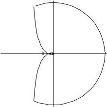
Figure 3.13 Map of the contour Γ under the map LDsE	3Ds 1E2
	sDs 6E2	, see D3.29E, which

is a conditionally stable system. The map of the positive imaginary axis is shown in full lines, the map of the negative imaginary axis and the small semicircle at the origin in dashed lines. The plot on the right is an enlargement of the area around the origin of the plot on the left.

result and appeared to require that all the steps be examined and set forth in full detail.

This quote clearly illustrate the difficulty in understanding feedback by simple qualitative reasoning. We will illustrate the issue of conditional stability by an example.

EXAMPLE 3.7—CONDITIONAL STABILITY

Consider a feedback system with the loop transfer function

	L s	E	3Ds 1E2	3.29
			sDs 6E2
	D			D E

The Nyquist plot of the loop transfer function is shown in Figure 3.13 The figure shows that the Nyquist curve intersects the negative real axis at a point close to -5. The naive argument would then indicate that the system would be unstable. The winding number is however zero and stability follows from Nyquist's theorem.

Notice that Nyquist's theorem does not hold if the loop transfer function has a pole in the right half plane. There are extensions of the Nyquist theorem to cover this case but it is simpler to invoke Theorem 1 directly. We illustrate this by two examples.

100

3.5 Frequency Response

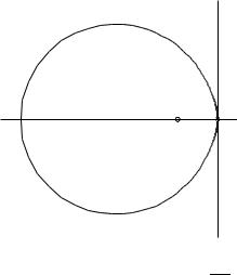
Figure 3.14 Map of the contour Γ under the map LDsE	k		. The curve on
	sDs−1EDs 5E

the right shows the region around the origin in larger scale. The map of the positive imaginary axis is shown in full lines, the map of the negative imaginary axis and the small semi circle at the origin in dashed lines.

EXAMPLE 3.8—LOOP TRANSFER FUNCTION WITH RHP POLE

Consider a feedback system with the loop transfer function

LDsE

k

sDs − 1EDs 5E

This transfer function has a pole at s 1 in the right half plane. This violates one of the assumptions for Nyquist's theorem to be valid. The Nyquist curve of the loop transfer function is shown in Figure 3.14. Traversing the contour Γ in clockwise we find that the winding number is 1. Applying Theorem 1 we find that

N − P 1

Since the loop transfer function has a pole in the right half plane we have P 1 and we get N 2. The characteristic equation thus has two roots in the right half plane.

EXAMPLE 3.9—THE INVERTED PENDULUM

Consider a closed loop system for stabilization of an inverted pendulum with a PD controller. The loop transfer function is

	L s	E	s 2	3.30
			s2 − 1
	D			D E
				101

s2−1

s 2

Chapter 3. Dynamics

Figure 3.15 Map of the contour Γ under the map LDsE given by D3.30E. The map of the positive imaginary axis is shown in full lines, the map of the negative imaginary axis and the small semi circle at the origin in dashed lines.

This transfer function has one pole at s 1 in the right half plane. The Nyquist curve of the loop transfer function is shown in Figure 3.15. Traversing the contour Γ in clockwise we find that the winding number is -1. Applying Theorem 1 we find that

N − P −1

Since the loop transfer function has a pole in the right half plane we have P 1 and we get N 0. The characteristic equation thus has no roots in the right half plane and the closed loop system is stable.

Bode Plots

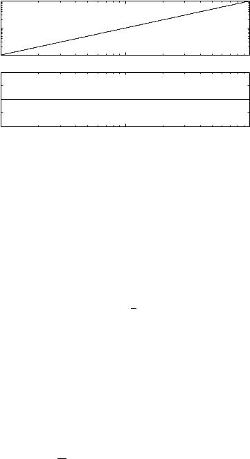
The Nyquist curve is one way to represent the frequency response GDiω E. Another useful representation was proposed by Bode who represented it by two curves, the gain curve and the phase curve. The gain curve gives the value of GDiω E as a function of ω and the phase curve gives arg GDiω E as a function of ω . The curves are plotted as shown below with logarithmic scales for frequency and magnitude and linear scale for phase, see Figure 3.16 An useful feature of the Bode plot is that both the gain curve and the phase curve can be approximated by straight lines, see Figure 3.16 where the approximation is shown in dashed lines. This fact was particularly useful when computing tools were not easily accessible.

102

3.5 Frequency Response

	105
GDiω Eh	104
	3
h	10
	102
	10−2	10−1	100	101

E	50
GDiω	0
	−50
arg	−100
	−150
	10−2	10−1	ω	100	101

Figure 3.16 Bode diagram of a frequency response. The top plot is the gain curve and bottom plot is the phase curve. The dashed lines show straight line approximations of the curves.

The fact that logarithmic scales were used also simplified the plotting. We illustrate Bode plots with a few examples.

It is easy to sketch Bode plots because with the right scales they have linear asymptotes. This is useful in order to get a quick estimate of the behavior of a system. It is also a good way to check numerical calculations.

Consider first a transfer function which is a polynomial GDsE BDsE/ADsE. We have

log GDsE log BDsE − log ADsE

Since a polynomial is a product of terms of the type :

s, s a, s2 2ζ as a2

it suffices to be able to sketch Bode diagrams for these terms. The Bode plot of a complex system is then obtained by composition.

EXAMPLE 3.10—BODE PLOT OF A DIFFERENTIATOR

Consider the transfer function

GDsE s

103

Chapter 3.		Dynamics
Eh	101
iω	0
	10
hGD
	10−1
	10−1	100	101
E	91
Diω	90.5
	90
G
arg	89.5
	89
	10−1	100	101
		ω

Figure 3.17 Bode plot of a differentiator.

We have GDiω E iω which implies

log hGDiω Eh log ω arg GDiω E π /2

The gain curve is thus a straight line with slope 1 and the phase curve is a constant at 90'.. The Bode plot is shown in Figure 3.17

EXAMPLE 3.11—BODE PLOT OF AN INTEGRATOR

Consider the transfer function

GDsE

1

s

We have GDiω E 1/iω which implies

log hGDiω Eh − log ω arg GDiω E −π /2

The gain curve is thus a straight line with slope -1 and the phase curve is a constant at −90'. The Bode plot is shown in Figure 3.18 Compare the Bode plots for the differentiator in Figure 3.17 and the integrator in Figure 3.18. The sign of the phase is reversed and the gain curve is mirror imaged in the horizontal axis. This is a consequence of

the property of the logarithm.

lon G1 −lonG −lonhGh − i arg G

104

3.5 Frequency Response

Eh		101
iω		0
		10
hGD
		10−1
		10−1	100	101
E		−89
Diω	−89.5
		−90
G
arg	−90.5
		−91
		10−1	100	101
			ω

Figure 3.18 Bode plot of an integrator.

EXAMPLE 3.12—BODE PLOT OF A FIRST ORDER FACTOR

Consider the transfer function

GDsE s a

We have

GDiω E a iω

and it follows that

p

hGDiω Eh ω 2 a2, arg GDiω E arctan ω /a

Hence

log hGDiω Eh 12 log Dω 2 a2E, arg GDiω E arctanω /a

The Bode Plot is shown in Figure 3.19. Both the gain curve and the phase curve can be approximated by straight lines if proper scales are chosen

105

Chapter 3. Dynamics

hGDiω Eh	101
	100
	10−1	100	101
Diω E	100
	50
arg G
	0
	10−1	100	101
		ω

Figure 3.19 Bode plot of a first order factor. The dashed lines show the piece-wise linear approximations of the curves.

and we obtain the following approximations.

log

G iω

8log a

T

if ω a, ,

>

<

h

D

Eh >log a log

2

if ω a,

:

if ω a

>log ω

1

ω

8π

if ω

a,

>0

>

>

<π

2

a

arg G

iω

>

4

if ω

a, ,

>

log

D

E

>

>

>

>

>

if ω a

:

2

>

Notice that a first order system behaves like an integrator for high frequencies. Compare with the Bode plot in Figure 3.18.

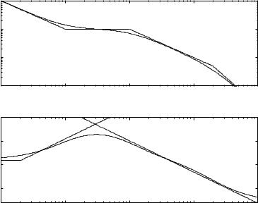
EXAMPLE 3.13—BODE PLOT OF A SECOND ORDER SYSTEM

Consider the transfer function

GDsE s2 2aζ s a2

We have

GDiω E a2 − ω 2 2iζ aω

106

3.5 Frequency Response

Hence

log hGDiω Eh 12 log Dω 4 2a2ω 2D2ζ 2 − 1E a4E arg GDiω E arctan 2ζ aω /Da2 − ω 2E

Notice that the smallest value of the magnitude minω hGDiω Eh 1/2ζ is obtained for ω a The gain is thus constant for small ω . It has an asymptote with zero slope for low frequencies. For large values of ω the gain is proportional to ω 2, which means that the gain curve has an asymptote with slope 2. The phase is zero for low frequencies and approaches 180' for large frequencies. The curves can be approximated with the following piece-wise linear expressions

>

2 log a

if ω a,

h

D

Eh

<

iω

>

log 2ζ

if ω

a, ,

log

G

82 log a

:

if ω a

>2 log ω

a

8π ω

if ω

a,

>0

>

<

−

if ω a,

D

iω

E

>

2

aζ

,

arg G

>

>

>

:

if ω a

>π

The Bode Plot is shown in Figure 3.20, the piece-wise linear approximations are shown in dashed lines.

Sketching a Bode Plot

It is easy to sketch the asymptotes of the gain curves of a Bode plot. This is often done in order to get a quick overview of the frequency response. The following procedure can be used

∙Factor the numerator and denominator of the transfer functions.

∙The poles and zeros are called break points because they correspond to the points where the asymptotes change direction.

∙Determine break points sort them in increasing frequency

∙Start with low frequencies

∙Draw the low frequency asymptote

∙Go over all break points and note the slope changes

107

Chapter 3. Dynamics

Eh	102
	101
GDiω	100
h
	10−1
	10−1	100	101
E	200
Diω	150
	100
G
arg	50
	0
	10−1	100	101
		ω

Figure 3.20 Bode plot of a second order factor with ζ 0.05 DdottedE, 0.1, 0.2, 0.5 and 1.0 Ddash-dottedE. The dashed lines show the piece-wise linear approximations of the curves.

∙A crude sketch of the phase curve is obtained by using the rela-

tion that, for systems with no RHP poles or zeros, one unit slope corresponds to a phase of 90'

We illustrate the procedure with the transfer function

G s		200Ds 1E		1 s
D	E	sDs 10EDs 200E		10sD1 0.1sED1 0.01sE

The break points are 0.01, 0.1, 1. For low frequencies the transfer function can be approximated by

GDsE

1

10s

Following the procedure we get

∙The low frequencies the system behaves like an integrator with gain

0.1. The low frequency asymptote thus has slope -1 and it crosses the axis of unit gain at ω 0.1.

∙The first break point occurs at ω 0.01. This break point corresponds to a pole which means that the slope decreases by one unit to -2 at that frequency.

∙The next break point is at ω 0.1 this is also a pole which means that the slope decreases to -3.

108

3.5 Frequency Response

100		Gain
10−1
10−2
10−3
10−1	100	101	102	103
		ω
0		Phase
−50
−100
−150
10−1	100	101	102	103
		ω

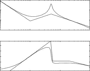
Figure 3.21 Illustrates how the asymptotes of the gain curve of the Bode plot can be sketched. The dashed curves show the asymptotes and the full lines the complete plot.

∙The next break point is at ω 1, since this is a zero the slope increases by one unit to -2.

Figure 3.21 shows the asymptotes of the gain curve and the complete Bode plot.

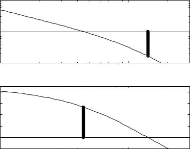
Gain and Phase Margins

The gain and phase margins can easily be found from the Bode plot of the loop transfer function. Recall that the gain margin tells how much the gain has to be increased for the system to reach instability. To determine the gain margin we first find the frequency ω pc where the phase is −180'. This frequency is called the phase crossover frequency. The gain margin is the inverse of the gain at that frequency. The phase margin tells how the phase lag required for the system to reach instability. To determine the phase margin we first determine the frequency ω nc where the gain of the loop transfer function is one. This frequency is called the gain crossover frequency. The phase margin is the phase of the loop transfer function

109

Chapter 3. Dynamics

101	gain
100
10−1
10−1	100
	phase

−100
−120
−140
−160
−180
−200
10−1	100

Figure 3.22 Finding gain and phase margins from the Bode plot of the loop transfer function.

at that frequency plus 180'. Figure 3.22 illustrates how the margins are found in the Bode plot of the loop transfer function.

Bode's Relations

Analyzing the Bode plots in the examples we find that there appears to be a relation between the gain curve and the phase curve. Consider e.g. the curves for the differentiator in Figure 3.17 and the integrator in Figure 3.18. For the differentiator the slope is 1 and the phase is constant pi/2 radians. For the integrator the slope is -1 and the phase is −pi/2. Bode investigated the relations between the curves and found that there was a unique relation between amplitude and phase for many systems. In particular he found the following relations for system with no

110

3.5

Frequency Response

poles and zeros in the right half plane.

ω 2 − ω 02

D

E

π

Z0

arg G

iω 0

2ω 0

[

log hGDiω Eh − log hGDiω 0Eh

dω

Z0

1

[ d log G

iω

ω

−

ω 0

h

D

Eh

log

ω

ω 0

d

π

h

D

iω

Eh

π

d log

ω

d log

G

2

d log ω

Z0

log

G

iω

2ω 2

[ ω −1 arg G

iω

ω −1 arg G

iω

h

D

Eh

−

0

D

E −

0

D

0Edω

log hGDiω 0Eh

π

ω 2 − ω 02

2ω 2

Z

[ d ω −1 arg G

iω

E log

ω

−

ω 0

−

0

dω

π

0

dω

D

ω

ω 0

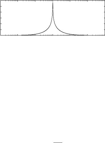
D3.31E The formula for the phase tells that the phase is a weighted average of the logarithmic derivative of the gain, approximatively

arg G	iω	E	π	d log hGDiω Eh	3.32
D			2 d log ω		D E

This formula implies that a slope of 1 corresponds to a phase of π /2, which holds exactly for the differentiator, see Figure 3.17. The exact formula D3.31E says that the differentiated slope should be weighted by the

kernel	Z0	[		ω	−		π 2
					ω 0
		log		ω	ω 0		dω 2

Figure 3.23 is a plot of the kernel.

Minimum Phase and Non-minimum Phase

Bode's relations hold for systems that do not have poles and zeros in the left half plane. Such systems are called minimum phase systems. One nice property of these systems is that the phase curve is uniquely given by the gain curve. These systems are also relatively easy to control. Other systems have larger phase lag, i.e. more negative phase. These systems are said to be non-minimum phase, because they have more phase lag than the equivalent minimum phase systems. Systems which do not have minimum phase are more difficult to control. Before proceeding we will give some examples.

EXAMPLE 3.14—A TIME DELAY

The transfer function of a time delay of T units is

GDsE e−sT

111

Chapter 3. Dynamics

				Weight
	6
	5
	4
y	3
	2
	1
	0
	10−3	10−2	10−1	100	101	102	103
				x

Figure 3.23 The weighting kernel in Bodes formula for computing the phase from the gain.

This transfer function has the property

hGDiω Eh 1, arg GDiω E −ω T

Notice that the gain is one. The minimum phase system which has unit gain has the transfer function GDsE 1. The time delay thus has an additional phase lag of ω T. Notice that the phase lag increases with increasing frequency. Figure 3.24 It seems intuitively reasonable that it is not possible to obtain a fast response of a system with time delay. We will later show that this is indeed the case.

Next we will consider a system with a zero in the right half plane

EXAMPLE 3.15—SYSTEM WITH A RHP ZERO

Consider a system with the transfer function

GDsE

a − s

a s

This transfer function has the property

hGDiω Eh 1, arg GDiω E −2 arctan ωa

Notice that the gain is one. The minimum phase system which has unit gain has the transfer function GDsE 1. In Figure 3.25 we show the Bode plot of the transfer function. The Bode plot resembles the Bode plot for a time delay which is not surprising because the exponential function e−sT

112

3.5 Frequency Response

101	Gain
100
10−1
10−1	100	101
	ω
	Phase
0
−100
−200
−300
−400
10−1	100	101
	ω

Figure 3.24 Bode plot of a time delay which has the transfer function GDsE e−s.

can be approximated by

e−sT 1 − sT/2 1 sT/2

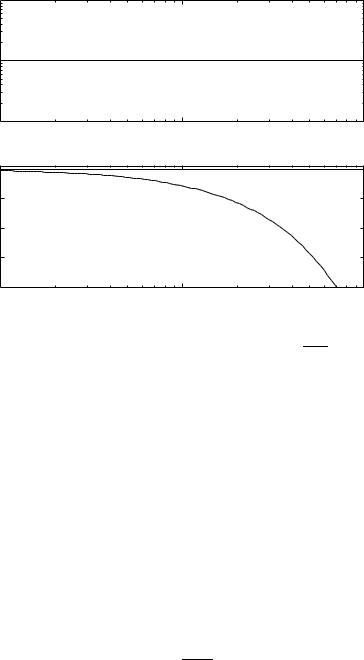
The largest phase lag of a system with a zero in the RHP is however pi. We will later show that the presence of a zero in the right half plane severely limits the performance that can be achieved. We can get an intuitive feel for this by considering the step response of a system with a right half plane zero. Consider a system with the transfer function GDsE that has a zero at s −α in the right half plane. Let h be the step response

of the system. The Laplace transform of the step response is given by

HDsE GDsE Z t e−st hDtEdt

s 0

113

Chapter 3. Dynamics

101	Gain
100
10−1
10−1	100		101
	ω
	Phase
0
−100
−200
−300
−400
10−1	100		101
	ω
Figure 3.25	Bode plot of a the transfer function G s	E	a − s .
	D		a s

Since GDα E is zero we have

Z t

0 e−α thDtEdt

0

Since e−α t is positive it follows that the step response hDtE must be negative for some t. This is illustrated in Figure 3.26 which shows the step response of a system having a zero in the right half plane. Notice that the output goes in the wrong direction initially. This is sometimes referred to as inverse response. It seems intuitively clear that such systems are difficult to control fast. This is indeed the case as will be shown in Chapter 5. We have thus found that systems with time delays and zeros in the right half plane have similar properties. Next we will consider a system with a right half plane pole.

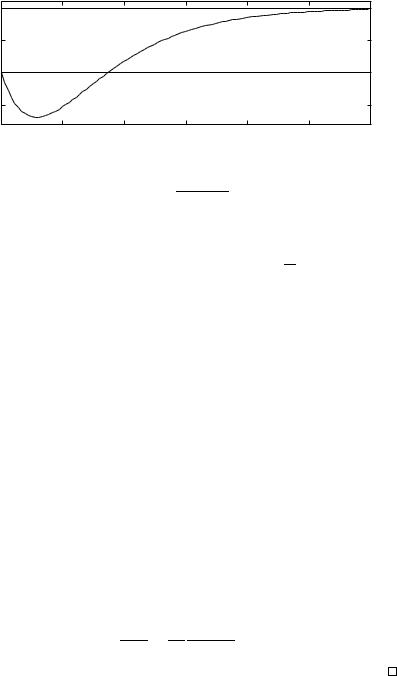
EXAMPLE 3.16—SYSTEM WITH A RHP POLE

Consider a system with the transfer function

GDsE

s a

s − a

114

3.5 Frequency Response

1
0.5
0
−0.5
0	0.5	1	1.5	2	2.5	3

Figure 3.26 Step response of a system with a zero in the right half plane. The

6D−s 1E system has the transfer function GDsE s2 5s 6 .

This transfer function has the property

a hGDiω Eh 1, arg GDiω E −2 arctan ω

Notice that the gain is one. The minimum phase system which has unit gain has the transfer function GDsE 1. In Figure 3.27 we show the Bode plot of the transfer function. Comparing the Bode plots for systems with a right half plane pole and a right half plane zero we find that the additional phase lag appears at high frequencies for a system with a right half plane zero and at low frequencies for a system with a right half plane pole. This means that there are significant differences between the systems. When there is a right half plane pole high frequencies must be avoided by making the system slow. When there is a right half plane zero low frequencies must be avoided and it is necessary to control these systems rapidly. This will

be discussed more in Chapter 5.

It is a severe limitation to have poles and zeros in the right half plane. Dynamics of this type should be avoided by redesign of the system. The zeros of a system can also be changed by moving sensors or by introducing additional sensors. Unfortunately systems which are non-minimum phase are not uncommon i real life. We end this section by giving a few examples.

EXAMPLE 3.17—HYDRO ELECTRIC POWER GENERATION

The transfer function from tube opening to electric power in a hydroelectric power station has the form

PDsE P0 1 − 2sT

ADsE A0 1 sT

where T is the time it takes sound to pass along the tube.

115

Chapter 3. Dynamics

101	Gain
100
10−1
10−1	100			101
	ω
	Phase
0
−50
−100
−150
10−1	100			101
	ω
Figure 3.27	Bode plot of a the transfer function G s	E	s a	which has a pole
	D		s − a

in the right half plane.

EXAMPLE 3.18—LEVEL CONTROL IN STEAM GENERATORS

Consider the problem of controlling the water level in a steam generator. The major disturbance is the variation of steam taken from the unit. When more steam is fed to the turbine the pressure drops. There is typically a mixture of steam and water under the water level. When pressure drops the steam bubbles expand and the level increases momentarily. After some time the level will decrease because of the mass removed from the system.

EXAMPLE 3.19—FLIGHT CONTROL

The transfer function from elevon to height in an airplane is non-minimum phase. When the elevon is raised there will be a force that pushes the rear of the airplane down. This causes a rotation which gives an increase of the angle of attack and an increase of the lift. Initially the aircraft will however loose height. The Wright brothers understood this and used control surfaces in the front of the aircraft to avoid the effect.

116