04.Multiport circuit parameters and transmission lines

Radio Frequency Circuit Design. W. Alan Davis, Krishna Agarwal

Copyright 2001 John Wiley & Sons, Inc.

Print ISBN 0-471-35052-4 Electronic ISBN 0-471-20068-9

CHAPTER FOUR

Multiport Circuit Parameters

and Transmission Lines

4.1VOLTAGE–CURRENT TWO-PORT PARAMETERS

A linear n-port network is completely characterized by n independent excitation variables and n dependent response variables. These variables are the terminal voltages and currents. There are four ways of arranging these independent and dependent variables for a two-port, and they are particularly useful, when considering feedback circuits. They are the impedance parameters (z-matrix), admittance parameters (y-matrix), hybrid parameters (h-matrix), and the inverse hybrid parameters (g-matrix). These four sets of parameters are defined as.

v2	D	z21	z22	i2	4.1
v1		z11	z12	i1
i2	D	y21	y22	v2	4.2
i1		y11	y12	v1
i2	D	h21	h22	v2	4.3
v1		h11	h12	i1
v2	D	g21	g22	i2	4.4
i1		g11	g12	v1

Two networks connected in series (Fig. 4.1) can be combined by simply adding the z parameters of each network together. This configuration is called the series–series connection. In the shunt–shunt configuration shown in Fig. 4.2, the two circuits can be combined by adding their y-matrices together. In the series–shunt configuration (Fig. 4.3), the composite matrix for the combination is found by adding the h parameters of each circuit together. Finally, the circuits

51

52 MULTIPORT CIRCUIT PARAMETERS AND TRANSMISSION LINES

Z G Z1

						Z L [Zc] = [Z1] + [Z2]
+
VG			Z2
–

FIGURE 4.1 Series–series connection.

		Y1
I G	Y G	Y L [Y c] = [Y 1] + [Y 2]
		Y2

FIGURE 4.2 Shunt–shunt connection.

Z G H 1

		Y L [H c ] = [H 1] + [H 2]
+
VG	H 2
–

FIGURE 4.3 Series–shunt connection.

connected in the shunt–series configuration (Fig. 4.4) can be combined by adding the g parameters of the respective circuits. In each type of configuration the independent variables are the same for the individual circuits, so matrix addition is valid most of the time. The case where the matrix addition is not valid occurs when for example in Fig. 4.1 a current going in and out of port 1 of circuit 1 is not equal to the current going in and out of port 1 of circuit 2. These pathological cases will not be of concern here, but further information is found in [1, pp. 188–191] where a description of the Brune test is given.

Any of the four types of circuit parameters described above can be represented by an equivalent circuit with controlled sources. As an example, the impedance (or z) parameters can be represented as shown in Fig. 4.5. The input port-1 side is represented by a series resistance of value z11 together with a current controlled

				ABCD PARAMETERS 53
			G1
i G						Z L [G c] = [G1] + [G 2]
		Y G
			G 2

FIGURE 4.4 Shunt–series connection.

i 1	Z 11							Z 22
								i 2
+								+
			+	+
v1	i 2Z 12				i		Z	v 2
			–	–		1		21
–								–
	FIGURE 4.5	Equivalent circuit for the z parameters.

voltage source with gain z12 in series. The controlling current is the port-2 current. If the current at port-1 is i1 and the current at port-2 is i2, then the voltage at port-1 is

v1 D i1z11 C i2z12

A similar representation is used for the port-2 side.

The individual impedance parameters are found for a given circuit by setting i1 or i2 to 0 and solving for the appropriate z parameter. The z parameters are sometimes termed open circuit parameters for this reason. The y parameters are sometimes called short circuit parameters because they are found by shorting the appropriate port. These parameters are all summarized in Appendix D where conversions are given for converting them to scattering parameters.

4.2ABCD PARAMETERS

Networks are often cascaded together, and it would be useful to be able to describe each network in such a way that the product of the matrices of each individual network would describe the total composite network. The ABCD parameters have the property of having the port-1 variables being the independent variables and the port-2 variables being the dependent ones:

54 MULTIPORT CIRCUIT PARAMETERS AND TRANSMISSION LINES

i1	D	C D	i2	4.5
v1		A B	v2

This allows the cascade of two networks to be represented as the matrix product of the two circuit expressed in terms of the ABCD parameters. The ABCD parameters can be expressed in terms of the commonly used z parameters:

A D v2 i2

0

D z21

4.6

v1

D

z11

B D

v1

v2

0 D

z

4.7

i2

D

z21

i1

1

C D

i2

0 D

4.8

v2

D

z21

D D

i1

v2

0 D

z22

4.9

i2

D

z21

where

z D z11z22 z21z12

In addition, if the circuit is reciprocal so that z12 D z21, then the determinate of the ABCD matrix is unity, namely

AD BC D 1

4.10

4.3IMAGE IMPEDANCE

A generator impedance is said to be matched to a load when the generator can deliver the maximum power to the load. This occurs when the generator impedance is the complex conjugate of the load impedance. For a two-port circuit, the generator delivers power to the circuit, which in turn has a certain load impedance attached to the other side (Fig. 4.6). Consequently maximum power transfer from the generator to the input of the two-port circuit occurs when it has the appropriate load impedance, ZL. The optimum generator impedance

	Z11
	i1	–i2
	ZG
	+	+
v1	A B C D	v 2	Z L = Z12
	–	–

FIGURE 4.6 Excitation of a two-port at port-1.

IMAGE IMPEDANCE

55

depends on both the two-port circuit itself and its load impedance. In addition the matched load impedance at the output side will depend on the two-port as well as on the generator impedance on the input side. Both sides are matched simultaneously when the input side is terminated with an impedance equal to its image impedance, ZI1, and the output side is terminated with a load impedance equal to ZI2. The actual values for ZI1, and ZI2 are determined completely by the two-port circuit itself and are independent of the loading on either side of the circuit. Terminating the two-port circuit in this way will guarantee maximum power transfer from the generator into the input side and maximum power transfer from a generator at the output side (if it exists).

The volt–ampere equations for a two-port are given in terms of their ABCD parameters as

v1 D Av2 Bi2	4.11
i1 D Cv2 Di2	4.12
Now, if the input port is terminated by ZI1 D v1/i1, and the output	port by

ZI2 D v2/ i2 , then both sides will be matched. Taking the ratios of Eqs. (4.11) and (4.12) gives

Z		v1			Av2/ i2		C B
I1	D	i1	D		Cv2/ i2		C D
		AZI2		C B			4.13
	D CZI2			C D

The voltage and current for the output side in terms of these parameters of the input side are found by inverting Eqs. (4.11) and (4.12):

v2 D Dv1 Bi1	4.14
i2 D Cv1 Ai1	4.15

If the output port is excited by v2 as shown in Fig. 4.7, then the matched load impedance is the same as the image impedance:

	Z		v2		Dv1/ i1	C B		DZI1 C B	4.16
		D i2		D Cv1/ i1		C A D CZI1 C A
	I2

Equations (4.13) and (4.16) can be solved to find the image impedances for both sides of the circuit:

AB

ZI1 D 4.17

CD

DB

ZI2 D 4.18

AC

56 MULTIPORT CIRCUIT PARAMETERS AND TRANSMISSION LINES

			Z 12
		i 1	–i 2	Z 12
	+			+
Z G = Z11	v1	A B C D		v 2
	–			–

FIGURE 4.7 Excitation of a two-port at port-2.

When a two-port circuit is terminated on each side by its image impedance so that ZG D ZI1 and ZL D ZI2, then the circuit is matched on both sides simultaneously. The input impedance is ZI1 if the load impedance is ZI2, and vice versa.

The image impedance can be written in terms of the open circuit z parameters and the short circuit y parameters by making the appropriate substitutions for the ABCD parameters (see Appendix D):

ZI1	D		y11		4.19
			z11
ZI2	D				4.20
			y22
			z22

Therefore an easy way to remember the values for the image impedances is

ZI1	D p			4.21
			zoc1zsc1
ZI2	D p			4.22
		zoc2zsc2

where zoc1 and zsc1 are the input impedances of the two-port circuit when the output port is an open circuit or a short circuit, respectively.

As an example consider the simple T circuit in Fig. 4.8. The input impedance when the output is an open circuit is

zoc1 D Za C Zb		4.23
Z a	Z c
	Z b

FIGURE 4.8 Example T circuit.

IMAGE IMPEDANCE

57

and the input impedance when the output is a short circuit is

zsc1 D Za C ZbjjZc

4.24

The image impedance for the input port for this circuit is

ZI1 D Za C Zb [Zc C ZbjjZc] 4.25

and similarly for the output port

ZI2 D Zc C Zb [Zc C ZbjjZa] 4.26

The output side of the two-port circuit can be replaced by another two-port whose input impedance is ZI2. This is possible if ZI2 is the image impedance of the second circuit and the load of the second circuit is equal to its output image impedance, say ZI3. A cascade of two-port circuits where each port is terminated by its image impedance would be matched everywhere (Fig. 4.9). A wave entering from the left side could propagate through the entire chain of two-port circuits without any internal reflections. There of course could be some attenuation if the two-port circuits contain lossy elements.

The image propagation constant, , for a two-port circuit is defined as

e D	v1i1	D	v1		ZI2	4.27
	v2 i2		v2		ZI1

If the network is symmetrical so that ZI1 D ZI2, then e D v1/v2. For the general unsymmetrical network, the ratio v1/v2 is found from Eq. (4.11) as

v1

D

Av2 Bi2

v2

v2

D A C

B

ZI2

D A C B

BD

AC

D

pAD C pBC

D

A

Z 12

Z 13

Z 14

Z 15

Z 16

Z 11

Z 16

1 2

2

3

3

4

4

5

5

6

FIGURE 4.9 Chain of matched two-port circuits.

58 MULTIPORT CIRCUIT PARAMETERS AND TRANSMISSION LINES

Similarly

i1	D CZI2 C D
i2
	D			A		pAD C pBC
				D

The image propagation constant is obtained from Eq. (4.27):

e D

v2

1

i2

D pAD C pBC

4.28

v i1

Also

e

p

p

D

AD

BC

4.29

When the circuit is reciprocal, AD BC D 1. Now if

Eqs. (4.28) and (4.29)

are added together and then subtracted from one another, the image propagation constant can be expressed in terms of hyperbolic functions:

	cosh D	p				4.30
				AD
		p
	sinh D			BC		4.31

If n represents the square root of the image impedance ratio, the ABCD parameters can then be written in terms of n and :

n D					ZI2
					ZI1
D										4.32
				D
				A
A D n cosh										4.33
B D nZI2 sinh										4.34
C D		sinh								4.35
		nZI2
D D		cosh								4.36
				n

Hence, from the definition of the ABCD matrix (4.5), the terminal voltages and currents can be written in terms of n and :

v1	D nv2 cosh ni2ZI2 sinh					4.37
		v2		i2
i1	D		sinh		cosh	4.38
		nZI2		n

THE TELEGRAPHER’S EQUATIONS

59

Division of these two equations gives the input impedance of the two-port circuit when it is terminated by ZL:

	Z		v1		n2Z		ZL C ZI2 tanh	4.39
		in D i1		D		I2 ZL tanh C ZI2

This is simply the transmission line equation for a lumped parameter network when the output is terminated by ZL D v2/ i2 . A clear distinction should be drawn between the input impedance of the network, Zin, which depends on the value of ZL, and the image impedance ZI2, which depends only on the twoport circuit itself. For a standard transmission line, ZI1 D ZI2 D Z0, where Z0 is the characteristic impedance of the transmission line. Just as for the image impedance, the characteristic impedance does not depend on the terminating impedances, but is a function of the geometrical features of the transmission line. When the lumped parameter circuit is lossless, D jˇ is pure imaginary and the hyperbolic functions become trigonometric functions:

	Z	n2Z		ZL C jZI2 tan ˇ	4.40
			I2 ZI2 C jZL tan ˇ
	in D

where ˇ is real. For a lossless transmission line of electrical length D ωL/v,

	Z	Z		ZL C jZ0 tan	4.41
			0 Z0 C jZL tan
	in D

where ω is the radian frequency, L is the length of the transmission line, and v is the velocity of propagation in the transmission line medium.

4.4THE TELEGRAPHER’S EQUATIONS

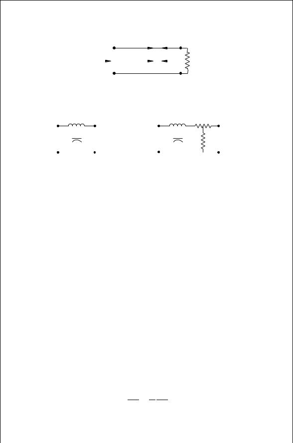
A transmission line consists of two conductors that are spaced somewhat less than a wavelength apart. The transmission line is assumed to support only a transverse electromagnetic (TEM) wave. The transmission line might support higher-order modes at higher frequencies, but it is assumed here that only the TEM wave is present. This assumption applies to the vast number of two conductor transmission lines used in practice. A transmission line may take a wide variety of forms; here it will be presented as a two-wire transmission line (Fig. 4.10). This line is represented as having a certain series inductance per unit length, L, and a certain shunt capacitance per unit length, C (Fig. 4.11). The inductance for the differential length is thus Ldz, and the capacitance is Cdz. If the incoming voltage and current wave entering port 1 is V D v1 and I D i1, respectively, then the voltage at port 2 is

∂V v2 D V C dz

∂z

60 MULTIPORT CIRCUIT PARAMETERS AND TRANSMISSION LINES

	+		+
Z		Z 0 V +				V –		ZL
		–				–
	z = –L					z = 0

FIGURE 4.10 Two wire representation of a transmission line.

Ldz

Ldz

Rdz

+

+

∂V

+

+

∂V

V1 = V Cdz

V1 = V

Cdz V2 = V +

∂z

dz

Gdz V2 = V +

∂z

dz

–

–

–

–

(a )

(b)

FIGURE 4.11 Circuit model of a differential length of a transmission line where (a) is the lossless line and (b) is the lossy line.

so the voltage difference between ports 1 and 2 is

	∂V		∂I	4.42
v2 v1 D		dz D Ldz
	∂z		∂t

The negative sign for the derivative indicates the voltage is decreasing in going from port-1 to port-2. Similarly the difference in current from port-1 to port-2 is the current going through the shunt capacitance:

		∂I						∂V		4.43
i2 i1 D					dz D Cdz
		∂z						∂t
The telegrapher’s equations are obtained from Eqs. (4.42) and (4.43):
	∂V			D L		∂I				4.44
	∂z					∂t

∂I ∂V

	D C		4.45
∂z		∂t

Differentiation of Eq. (4.44) with respect to z and Eq. (4.45) with respect to t, and then combining, produces the voltage wave equation:

∂2V 1 ∂2V	4.46
∂z2 D v2 ∂t2