5.Feedback fundamentals

5.3 The Gang of Six

1.4					Output
1.2
1
0.8
y
0.6
0.4
0.2
0	20	40	60	80	100	120	140	160	180	200
0
					Control

0
−0.2
−0.4
−0.6
u
−0.8
−1
−1.2
−1.4	20	40	60	80	100	120	140	160	180	200
0
					t

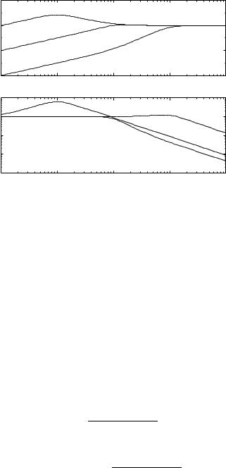
Figure 5.7 Response of output y and control u to a step in the load disturbance. Notice the very slow decay of the mode e−0.02t. The control signal does not respond to this mode because the controller has a zero s −0.02.

signal e−0.02t because the zero s −0.02 will block the transmission of this signal. This is clearly seen in Figure 5.7, which shows the response of the output and the control signals to a step change in the load disturbance. Notice that it takes about 200 s for the disturbance to settle. This can be compared with the step response in Figure 5.6 which settles in about 10s.

The behavior illustrated in the example is typical when there are cancellations of poles and zeros in the transfer functions of the process and the controller. The canceled factors do not appear in the loop transfer function and the sensitivity functions. The canceled modes are not visible unless they are excited. The effects are even more drastic than shown in the example if the canceled modes are unstable. This has been known among control engineers for a long time and a there has been a design rule that cancellation of slow or unstable modes should be avoided. Another view of cancellations is given in Section 3.7.

187

Chapter 5.	Feedback Fundamentals
					d				n
	r 0		C	u	Σ	P	x	Σ		yol
					d					n
r 0	Σ	e	C	u	Σ	P		x	Σ	ycl

−1

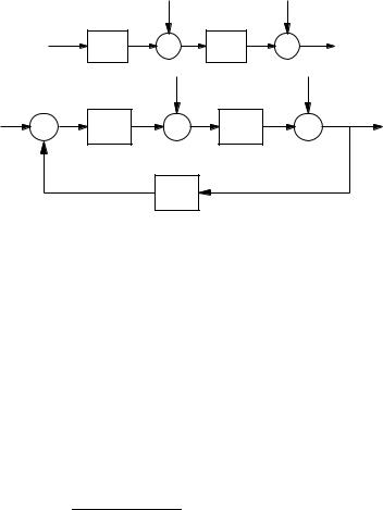
Figure 5.8 Open and closed loop systems subject to the same disturbances.

5.4 Disturbance Attenuation

The attenuation of disturbances will now be discussed. For that purpose we will compare an open loop system and a closed loop system subject to the disturbances as is illustrated in Figure 5.8. Let the transfer function of the process be PDsE and let the Laplace transforms of the load disturbance and the measurement noise be DDsE and NDsE respectively. The output of the open loop system is

Yol PDsEDDsE NDsE

D5.4E

and the output of the closed loop system is

	Y	PDsEDDsE NDsE		S s	ED	P s	D s	E	N s	EE	5.5
		1 PDsECDsE
	cl			D		D E	D		D		D E

where SDsE is the sensitivity function, which belongs to the Gang of Four. We thus obtain the following interesting result

YclDsE SDsEYolDsE

D5.6E

The sensitivity function will thus directly show the effect of feedback on the output. The disturbance attenuation can be visualized graphically by the gain curve of the Bode plot of SDsE. The lowest frequency where the sensitivity function has the magnitude 1 is called the sensitivity crossover frequency and denoted by ω sc. The maximum sensitivity

			1
Ms ω h D Eh	ω				D E
			1 PDiω ECDiω E
max S iω	max				5.7

188

5.4 Disturbance Attenuation

	101
hSDiω Eh	100
	10−1
	10−2	10−1		100	101
	10−2		ω
Figure 5.9 Gain curve of the sensitivity function for PI control Dk 0.8, ki 0.4E
of process with the transfer function PDsE Ds 1E−4. The sensitivity crossover

frequency is indicated by and the maximum sensitivity by o.

	30
	20
	10
y	0
	−10
	−20
	−30	10	20	30	40	50	60	70	80	90	100
	0
						t

Figure 5.10 Outputs of process with control Dfull lineE and without control Ddashed lineE.

is an important variable which gives the largest amplification of the disturbances. The maximum occurs at the frequency ω ms.

A quick overview of how disturbances are influenced by feedback is obtained from the gain curve of the Bode plot of the sensitivity function. An example is given in Figure 5.9. The figure shows that the sensitivity crossover frequency is 0.32 and that the maximum sensitivity 2.1 occurs at ω ms 0.56. Feedback will thus reduce disturbances with frequencies less than 0.32 rad/s, but it will amplify disturbances with higher frequencies. The largest amplification is 2.1.

If a record of the disturbance is available and a controller has been designed the output obtained under closed loop with the same disturbance can be visualized by sending the recorded output through a filter with the transfer function SDsE. Figure 5.10 shows the output of the system with and without control.

189

Chapter 5. Feedback Fundamentals

−1	ω ms
1/Ms
	ω sc

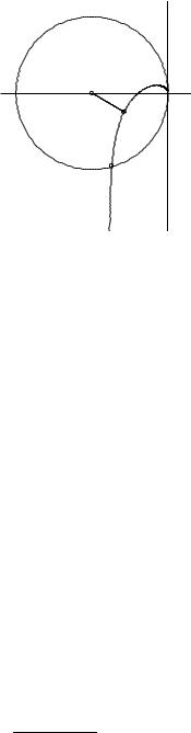
Figure 5.11 Nyquist curve of loop transfer function showing graphical interpretation of maximum sensitivity. The sensitivity crossover frequency ω sc and the frequency ω ms where the sensitivity has its largest value are indicated in the figure. All points inside the dashed circle have sensitivities greater than 1.

The sensitivity function can be written as
SDsE	1			1	.	D5.8E
	1 PDsECDsE			1 LDsE

Since it only depends on the loop transfer function it can be visualized graphically in the Nyquist plot of the loop transfer function. This is illustrated in Figure 5.11. The complex number 1 LDiω E can be represented as the vector from the point −1 to the point LDiω E on the Nyquist curve. The sensitivity is thus less than one for all points outside a circle with radius 1 and center at −1. Disturbances of these frequencies are attenuated by the feedback. If a control system has been designed based on a given model it is straight forward to estimated the potential disturbance reduction simply by recording a typical output and filtering it through the sensitivity function.

Slow Load Disturbances

Load disturbances typically have low frequencies. To estimate their effects on the process variable it is then natural to approximate the transfer function from load disturbances to process output for small s, i.e.

G

s

E

PDsE

c

c s

c s2

× × ×

5.9

1 PDsECDsE

xdD

0

1

2

D E

190

5.5 Process Variations

The coefficients ck are called stiffness coefficients. This means that the process variable for slowly varying load disturbances d is given by

x t	c d t	c	ddDtE		c	d2dDtE	× × ×
D E	0 D E	1 dt			2 dt2

For example if the load disturbance is dDtE v0t we get

xDtE c0v0t c1v0

If the controller has integral action we have c0 0 and xDtE c1v0.

5.5 Process Variations

Control systems are designed based on simplified models of the processes. Process dynamics will often change during operation. The sensitivity of a closed loop system to variations in process dynamics is therefore a fundamental issue.

Risk for Instability

Instability is the main drawback of feedback. It is therefore of interest to investigate if process variations can cause instability. The sensitivity functions give a useful insight. Figure 5.11 shows that the largest sensitivity is the inverse of the shortest distance from the point −1 to the Nyquist curve.

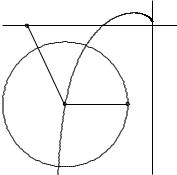
The complementary sensitivity function also gives insight into allowable process variations. Consider a feedback system with a process P and a controller C. We will investigate how much the process can be perturbed without causing instability. The Nyquist curve of the loop transfer function is shown in Figure 5.12. If the process is changed from P to P DP the loop transfer function changes from PC to PC CDP as illustrated in the figure. The distance from the critical point −1 to the point L is h1 Lh. This means that the perturbed Nyquist curve will not reach the critical point −1 provided that

hCDPh h1 Lh

This condition must be valid for all points on the Nyquist curve. The condition for stability can be written as

	hDPDiω Eh		1		D	5.10	E
	hPDiω Eh		hTDiω Eh
						191

Chapter 5. Feedback Fundamentals

−1
1 L
C	P

Figure 5.12 Nyquist curve of a nominal loop transfer function and its uncertainty caused by process variations P.

A technical condition, namely that the perturbation P is a stable transfer function, must also be required. If this does not hold the encirclement condition required by Nyquist's stability condition is not satisfied. Also notice that the condition D5.10E is conservative because it follows from Figure 5.12 that the critical perturbation is in the direction towards the critical point −1. Larger perturbations can be permitted in the other directions.

This formula D5.10E is one of the reasons why feedback systems work so well in practice. The mathematical models used to design control system are often strongly simplified. There may be model errors and the properties of a process may change during operation. Equation D5.10E implies that the closed loop system will at least be stable for substantial variations in the process dynamics.

It follows from D5.10E that the variations can be large for those frequencies where T is small and that smaller variations are allowed for frequencies where T is large. A conservative estimate of permissible pro-

cess variations that will not cause instability is given by
	h	PDiω Eh			1
	hPDiω Eh					Mt
where Mt is the largest value of the complementary sensitivity
Mt ω h D Eh ω						P iω C iω				D E
					1 DPDiEω EDCDiEω E
max T iω
		max								5.11

The value of Mt is influenced by the design of the controller. For example if Mt 2 gain variations of 50% and phase variations of 30' are permitted

192

5.5 Process Variations

without making the closed loop system unstable. The fact that the closed loop system is robust to process variations is one of the reason why control has been so successful and that control systems for complex processes can indeed be designed using simple models. This is illustrated by an example.

EXAMPLE 5.2—MODEL UNCERTAINTY

Consider a process with the transfer function

1

PDsE Ds 1E4

A PI controller with the parameters k 0.775 and Ti 2.05 gives a closed loop system with Ms 2.00 and Mt 1.35. The complementary sensitivity has its maximum for ω mt 0.46. Figure 5.13 shows the Nyquist curve of the transfer function of the process and the uncertainty bounds P hPh/hTh for a few frequencies. The figure shows that

∙ Large uncertainties are permitted for low frequencies, TD0E 1.

∙ The smallest relative error h P/Ph occurs for ω 0.46.

∙For ω 1 we have hTDiω Eh 0.26 which means that the stability requirement is h P/Ph 3.8

∙For ω 2 we have hTDiω Eh 0.032 which means that the stability requirement is h P/Ph 31

The situation illustrated in the figure is typical for many processes, moderately small uncertainties are only required around the gain crossover frequencies, but large uncertainties can be permitted at higher and lower frequencies. A consequence of this is also that a simple model that describes the process dynamics well around the crossover frequency is sufficient for design. Systems with many resonance peaks are an exception to this rule because the process transfer function for such systems may have large gains also for higher frequencies.

Variations in Closed Loop Transfer Function

So far we have investigated the risk for instability. The effects of small variation in process dynamics on the closed loop transfer function will now be investigated. To do this we will analyze the system in Figure 5.1. For simplicity we will assume that F 1 and that the disturbances d and n are zero. The transfer function from reference to output is given by

Y		PC	T	D5.12E
R		1 PC
				193

Chapter 5. Feedback Fundamentals

Figure 5.13 Nyquist curve of a nominal process transfer function PDsE Ds 1E−4 shown in full lines. The circles show the uncertainty regions h Ph 1/hTh obtained for a PI controller with k 0.775 and Ti 2.05 for ω 0, 0.46 and 1.

Compare with D5.2E. The transfer function T which belongs to the Gang of Four is called the complementary sensitivity function. Differentiating D5.12E we get

dT

C

PC

S

T

dP

D1 PCE2

D1 PCED1 PCEP

P

Hence

d log T

dT P

D5.13E

S

d log P

dP

T

This equation is the reason for calling S the sensitivity function. The relative error in the closed loop transfer function T will thus be small if the sensitivity is small. This is one of the very useful properties of feedback. For example this property was exploited by Black at Bell labs to build the feedback amplifiers that made it possible to use telephones over large distances.

A small value of the sensitivity function thus means that disturbances are attenuated and that the effect of process perturbations also are negligible. A plot of the magnitude of the complementary sensitivity function as in Figure 5.9 is a good way to determine the frequencies where model precision is essential.

194

5.5 Process Variations

Constraints on Design

Constraints on the maximum sensitivities Ms and Mt are important to ensure that closed loop system is insensitive to process variations. Typical constraints are that the sensitivities are in the range of 1.1 to 2. This has implications for design of control systems which are illustrated by an example.

EXAMPLE 5.3—SENSITIVITIES CONSTRAIN CLOSED LOOP POLES

PI control of a first order system was discussed in Section 4.4 where it was shown that the closed loop system was of second order and that the closed loop poles could be placed arbitrarily by proper choice of the controller parameters. The process and the controller are characterized by

YDsE s b a U DsE

U DsE −kYDsE ksi DRDsE − YDsEE

where U , Y and R are the Laplace transforms of the process input, output and the reference signal. The closed loop characteristic polynomial is

s2 Da bkEs bki

requiring this to be equal to

s2 2ζ ω 0s ω 02

we find that the controller parameters are given by

k 2ζ ω 0 − 1 b

ω 2 ki b0

and there are no apparent constraints on the choice of parameters ζ and ω 0. Calculating the sensitivity functions we get

	S s		sDs aE
		E s2 2ζ ω 0s ω 02
	D
	T s	E	D2ζ ω 0 − aEs ω 02
			s2 2ζ ω 0s ω 02
	D

195

Chapter 5. Feedback Fundamentals

	102
SDiω Eh	100
	−2
h
	10
	10−4	10−1	100	101	102
	10−2
			ω
	101
iωEh	100
	10−1
hSD
	10−2
	10−3	10−1	100	101	102
	10−2
			ω
Figure 5.14 Magnitude curve for bode plots of the sensitivity function DaboveE and
the complementary sensitivity function DbelowE for ζ				0.7, a 1 and ω0/a 0.1
DdashedE, 1 DsolidE and 10 DdottedE.

Figure 5.14 shows clearly that the sensitivities will be large if the parameter ω 0 is chosen smaller than a. The equation for controller gain also gives an indication that small values of ω 0 are not desirable because proportional gain then becomes negative which means that the feedback is positive.

Sensitivities and Relative Damping

For simple low order control systems we have based design criteria on the patterns of the poles and zeros of the complementary transfer function. To relate the general results on robustness to the analysis of the simple controllers it is of interest to find the relations between the sensitivities and relative damping. The complementary sensitivity function for a standard second order system is given by

ω 2

TDsE 0

s2 2ζ ω 0s ω 02

This implies that the sensitivity function is given by

	S s		1		T s	sDs 2ζ ω 0E
		E		−		E s2 2ζ ω 0s ω 02
	D				D

196