07.Frequency domain methods for stability

This version: 22/10/2004

Chapter 7

Frequency domain methods for stability

In Chapter 5 we looked at various ways to test various notions of stability of SISO control systems. Our stability discussion in that section ended with a discussion in Section 6.2.3 of how interconnecting systems in block diagrams a ects stability of the resulting system. The criterion developed by Nyquist [1932] deals further with testing stability in such cases, and we look at this in detail in this chapter. The methods in this chapter rely heavily on some basic ideas in complex variable theory, and these are reviewed in Appendix D.

Contents

7.1	The Nyquist criterion . . . . . . . . . . . . . . . . . . . . . . . . . . . . . . . . . . . . . .		279
	7.1.1 The Principle of the Argument . . . . . . . . . . . . . . . . . . . . . . . . . . . . .		279
	7.1.2 The Nyquist criterion for single-loop interconnections . . . . . . . . . . . . . . . .		281
7.2	The relationship between the Nyquist contour and the Bode plot . . . . . . . . . . . . . .		293
	7.2.1 Capturing the essential features of the Nyquist contour from the Bode plot . . . .		293
	7.2.2	Stability margins . . . . . . . . . . . . . . . . . . . . . . . . . . . . . . . . . . . .	294
7.3	Robust stability . . . . . . . . . . . . . . . . . . . . . . . . . . . . . . . . . . . . . . . . .		303
	7.3.1	Multiplicative uncertainty . . . . . . . . . . . . . . . . . . . . . . . . . . . . . . .	304
	7.3.2	Additive uncertainty . . . . . . . . . . . . . . . . . . . . . . . . . . . . . . . . . .	308
7.4	Summary . . . . . . . . . . . . . . . . . . . . . . . . . . . . . . . . . . . . . . . . . . . . .		311

7.1 The Nyquist criterion

The Nyquist criterion is a method for testing the closed-loop stability of a system based on the frequency response of the open-loop transfer function.

7.1.1 The Principle of the Argument In this section we review one of the essential tools in dealing with closed-loop stability as we shall in this chapter: the so-called Principle of the Argument. This is a result from the theory of complex analytic functions. That such technology should be useful to us has been made clear in the developments of Section 4.4.2 concerning Bode’s Gain/Phase Theorem. The Principle of the Argument has to do, as we shall use it, with the image of closed contours under analytic functions. However, let us first provide its form in complex analysis. Let U C be an open set, and let f : U → C be an analytic function. A pole for f is a point s0 U with the property that the limit

280

7 Frequency domain methods for stability

22/10/2004

lims→s0 f(s) does not exist, but there exists a k N so that the limit lims→s0 (s − s0)kf(s) does exist. Recall that a meromorphic function on an open subset U C is a function f : U → C having the property that it is defined and analytic except at isolated points (i.e., except at poles). Now we can state the Principle of the Argument, which relies on the Residue Theorem stated in Appendix D.

7.1 Theorem (Principle of the Argument) Let U be a simply connected open subset of C and let C be a contour in U. Suppose that f is a function which

(i)is meromorphic in U,

(ii)has no poles or zeros on the contour C, and

(iii)has np poles and nz zeros in the interior of C, counting multiplicities of zeros and poles.

Then	ZC	f0(s) ds = 2πi(nz − np),
		f (s)
provided integration is performed in a counterclockwise direction.
Proof Since f is meromorphic,	f0	is also meromorphic, and is analytic except at the poles
	f

and zeroes of f. Let s0 be such a pole or zero, and suppose that it has multiplicity k. Then there exists a meromorphic function f˜, analytic an s0, with the property that f(s) =

k ˜
(s − s0) f(s). One then readily determines that
	f0(s)	=	k	+	f˜0(s)
	f(s)		s − s0			f˜(s)

for s in a neighbourhood of s0. Now by the Residue Theorem the result follows since k is positive if s0 is a zero and negative if s0 is a pole.

The use we will make of this theorem is in ascertaining the nature of the image of a closed contour under an analytic function. Thus we let U C be an open set and c: [0, T ] → U a closed curve. The image of c we denote by C, and we let f be a function satisfying the hypotheses of Theorem 7.1. Let us denote by c˜ the curve defined by c˜(t) = f ◦ c(t). Since f has no zeros on C, the curve c˜ does not pass through the origin and so the function F : [0, T ] → C defined by F (t) = ln(˜c(t)) is continuous. By the chain rule we have

f0(c(t))

F 0(t) =

c0(t), t [0, T ].

f(c(t))

Therefore

f0(s) ds = ZC f0(c(t)) c0

(t) dt = ln(f(c(t))) 0 .

ZC

f (s)

f (c(t))

T

Using the definition of the logarithm we have

T

= ln |f(c(t))|

T

T

ln(f(c(t))) 0

0

+ i]f(c(t)) 0 .

Since c is closed, the first term on the right-hand side is zero. Using Theorem 7.1 we then have

T	(7.1)
2π(nz − np) = ]f(c(t)) 0 .

In other words, we have the following.

22/10/2004		7.1 The Nyquist criterion	281
7.2 Proposition If	C and	f are as in Theorem 7.1, then the image of	C under f encircles
the origin nz − np	times,	with the convention that counterclockwise is positive.

Let us illustrate the principle with an example.

7.3 Example We take C to be the circle of radius 2 in C. This can be parameterised, for example, by c: t 7→2eit, t [0, 2π]. For f we take

f(s) =	1	, a R.
	(s + 1)2 + a2

Let’s see what happens as we allow a to vary between 0 and 1.5. The curve c˜ = f ◦ c is

defined by
1
t 7→		, t [0, 2π].
	(e2it + 1)2 + a2

Proposition 7.2 says that for a < 1 the image of C should encircle the origin in C two times in the counterclockwise direction, and for a > 1 there should be no encirclements of the origin. Of course, it is problematic to determine the image of a closed contour under a given analytic function. Here we let the computer do the work for us, and the results are shown

in Figure 7.1. We see that the encirclements are as we expect.
7.1.2 The Nyquist criterion for single-loop interconnections	Now we apply the

Principle of the Argument to determine the stability of a closed-loop transfer function. The block diagram configuration we consider here is shown in Figure 7.2. The key observation is that if the system is to be IBIBO stable then the poles of the closed-loop transfer function

RC (s)RP (s)

T (s) = 1 + RC (s)RP (s)

must all lie in C−. The idea is that we examine the determinant 1 + RC RP to ascertain when the poles of T are stable.

We denote the loop gain by RL = RC RP . Suppose that RL has poles on the imaginary axis at ±iω1, . . . , ±iωk where ωk > · · · > ω1 ≥ 0. Let r > 0 have the property that

	1
r <			min	(7.2)
	2 i,j {1,...,k}{|ωi − ωj|}.
			i6=j

That is, r is smaller than half the distance separating the two closest poles on the imaginary
axis. Now we choose R so that	r
R > ωk +		.	(7.3)
	2

With r and R so chosen we may define a contour R,r which will be comprised of a collection

of components. For i = 1, . . . , k				we define		r,k,− = − iωi + reiθ
r,k,+ =	iωi + reiθ		− π2	≤ θ ≤ π2	,			− π2 ≤ θ ≤	π2 .
		define
Now for i = 1, . . . , k − 1
¯	| ωi + r < ω < ωi+1 − r} ,					¯	− ωi − r > ω > −ωi+1		+ r} ,
r,i,+ = {iω						r,i,− = {iω |
and also define
¯		ωk + r < ω < R} ,				¯	− ωk − r > ω > −R} .
r,i,+ = {iω |						r,i,− = {iω |

282		7 Frequency domain methods for stability		22/10/2004
	4		4
	3		3
	2		2
	1		1
Im	0	Im	0
	-1		-1
	-2		-2
	-3		-3

-3	-2	-1	0	1	2		3	4	-3		-2	-1	0	1	2	3	4
			Re										Re
				4
				3
				2
				1
			Im	0
				-1
				-2
				-3
					-3	-2	-1	0	1	2	3		4

Re

Figure 7.1 Images of closed contours for a = 0 (top left), a = 0.5 (top right), and a = 1.5 (bottom)

rˆ(s)	RC (s)	RP (s)	yˆ(s)
	−

Figure 7.2 A unity feedback loop

Finally we define

R = Reiθ − π2 ≤ θ ≤ π2 .

22/10/2004

7.1 The Nyquist criterion

283

The union of all these various contours we denote by R,r:

kk

[	i[	¯	¯	[
R,r = r,i,+ r,i,−		r,i,+ r,i,−		R.
i=1	=1

When RL has no poles on the imaginary axis, for R > 0 we write

[

R,0 = {iω | − R < ω < R} R.

Note that the orientation of the contour R,r is taken by convention to be positive in the clockwise direction. This is counter to the complex variable convention, and we choose this convention because, for reasons will soon see, we wish to move along the positive imaginary axis from bottom to top. In any case, the idea is that we have a semicircular contour extending into C+, and we need to make provisions for any poles of RL which lie on the imaginary axis. The situation is sketched in Figure 7.3. With this notion of a contour behind

Im

R

Re

Figure 7.3 The contour R,r

us, we can define what we will call the Nyquist contour.

7.4 Definition For the unity feedback loop of Figure 7.2, let RL be the rational function RC RP , and let R and r satisfy the conditions (7.3) and (7.2). The (R, r)-Nyquist contour is the contour RL( R,r) C. We denote the (R, r)-Nyquist contour by NR,r.

When we are willing to live with the associated imprecision, we shall often simply say “Nyquist contour” in place of “(R, r)-Nyquist” contour.

Let us first state some general properties of the (R, r)-Nyquist contour. At the same time we introduce some useful notation. Since we are interested in using the Nyquist criterion for determining IBIBO stability, we shall suppose RL to be proper, as in most cases we encounter.

¯

7.5 Proposition Let RL be a proper rational function, and for δ > 0 let D(0, δ) = {s C | |s| ≤ δ} be the disk of radius δ centred at the origin in C. The following statements hold.

284			7 Frequency domain methods for stability			22/10/2004
(i)	If	RL has no poles on the imaginary axis then there exists			M > 0 so that for any
	R > 0 the		(R, 0)-Nyquist contour is contained in the disk		¯	Furthermore
					D(0, M).
(ii)	limR→∞ NR,0		is well-defined and we denote the limit by N∞,0.
	If	RL is strictly proper, then for any		r > 0 satisfying (7.2) and for any		> 0 there
	exists R0 > 0 so that NR,r \ NR0,r			¯
				D(0, ) for any R > R0. Thus limR→∞ NR,r is

well-defined and we denote the limit by N∞,r.

(iii)If RL is both strictly proper and has no poles on the imaginary axis, then the consequences of (ii) hold with r = 0, and we denote by N∞,0 the limit limR→∞ NR,0.

Proof (i) Define R(s) = RL(1s ) for s 6= 0. Since RL is proper, the limit lims→0 R(s) exists. But, since RL is continuous, this is nothing more than the assertion we are trying to prove.

(ii) If RL is strictly proper then lims→∞ RL(s) = 0. Therefore, by continuity of RL we can choose R0 su ciently large that, for R > R0, those points which lie in the (R, r)-Nyquist

	¯
contour but do not lie in the (R0, r)-Nyquist contour reside in the disk D(0, ). This is
precisely what we have stated.
(iii) This is a simple consequence of (i) and (ii).

The punchline here is that the Nyquist contour is always bounded for proper loop gains, provided that there are no poles on the imaginary axis. When there are poles on the imaginary axis, then the Nyquist contour will be unbounded, but for any fixed r > 0 su ciently small, we may still consider letting R → ∞.

Let us see how the character of the Nyquist contour relates to stability of the closed-loop system depicted in Figure 7.2.

7.6 Theorem (Nyquist Criterion) Let RC and RP be rational functions with RL = RC RP proper. Let np be the number of poles of RL in C+. First suppose that 1+RL has no zeros on iR. Then the interconnected SISO linear system represented by the block diagram Figure 7.2 is IBIBO stable if and only if

(i)there are no cancellations of poles and zeros in C+ between RC and RP ;

(ii)lims→∞ RL(s) 6= −1;

(iii) there exists R0, r0 > 0 satisfying (7.3) and (7.2) with the property	that for every
R > R0 and r < r0, the (R, r)-Nyquist contour encircles the point	−1 + i0 in the
complex plane np times in the counterclockwise direction as the contour R,r is traversed
once in the clockwise direction.

Furthermore, if for any R and r satisfying (7.3) and (7.2) the (R, r)-Nyquist contour passes through the point −1 + i0, and in particular if 1 + RL has zeros on iR, then the closed-loop system is IBIBO unstable.

Proof We first note that the condition (ii) is simply the condition that the closed-loop transfer function be proper. If the closed-loop transfer function is not proper, then the resulting interconnection cannot be IBIBO stable.

By Theorem 6.38, the closed-loop system is IBIBO stable if and only if (1) all the closedloop transfer function is proper, (2) the zeros of the determinant 1 + RL are in C−, and

(3) there are no cancellations of poles and zeros in C+ between RC and RP . Thus the first statement in the theorem will follow if we can show that, when 1 + RL has no zeros on iR, the condition (iii) is equivalent to the condition

(iv) all zeros of the determinant 1 + RL are in C−.

22/10/2004

7.1 The Nyquist criterion

285

Since there are no poles or zeros of 1 + RL on R,r, provided that R > R0 and r < r0, we can apply Proposition 7.2 to the contour R,r and the function 1 + RL. The conclusion is that the image of R,r under 1 + RL encircles the origin nz − np times, with nz being the number of zeros of 1 + RL in C+ and np being the number of poles of 1 + RL in C+. Note that the poles of 1 + RL are the same as the poles of RL, so np is the same as in the statement of the theorem. The conclusion in this case is that nz = 0 if and only if the image of R,r under 1 + RL encircles the origin np times, with the opposite orientation of R,r. This, however, is equivalent to the image of R,r encircling −1 + i0 np times, with the opposite orientation of

R,r.

Finally, if the (R, r)-Nyquist contour passes through the point −1 + i0, this means that the contour 1 + RL( R,r) passes through the origin. Thus this means that there is a point

s0 R,r which is a zero of 1 + RL. However, since all points on R,r are in C+, the result follows by Theorem 6.38.

Let us make a few observations before working out a few simple examples.

7.7 Remarks 1. Strictly proper rational functions always satisfy the condition (ii).

2.Of course, the matter of producing the Nyquist contour may not be entirely a straightforward one. What one can certainly do is produce it with a computer. As we will see, the Nyquist contour provides a graphical representation of some important properties of the closed-loop system.

3.By parts (i) and (ii) of Proposition 4.13 it su ces to plot the Nyquist contour only as we traverse that half of R,r which sits in the positive imaginary plane, i.e., only for those values of s along R,r which have positive imaginary part. This will be borne out in the examples below.

4.When RL is proper and when there are no poles for RL on the imaginary axis (so we

can take r = 0), the (R, 0)-Nyquist contour is bounded as we take the limit R → ∞. If we further ask that RL be strictly proper, that portion of the Nyquist contour which is the image of R under RL will be mapped to the origin as R → ∞. Thus in this case it su ces to determine the image of the imaginary axis under RL, along with the origin in C. Given our remark 3, this essentially means that in this case we only determine the polar plot for the loop gain RL. Thus we see the important relationship between the Nyquist criterion and the Bode plot of the loop gain.

5. Here’s one way to determine the number of times the (R, r)-Nyquist contour encircles the point −1 + i0. From the point −1 + i0 draw a ray in any direction. Choose this ray so that it is nowhere tangent to the (R, r)-Nyquist contour, and so that it does not pass through points where the (R, r)-Nyquist contour intersects itself. The number of times the (R, r)-Nyquist contour intersects this ray while moving in the counterclockwise direction is the number of counterclockwise encirclements of −1 + i0. A crossing in the clockwise direction is a negative counterclockwise crossing.

The Nyquist criterion can be readily demonstrated with a couple of examples. In each of these examples we use Remark 7.7–(5).

In the Nyquist plots below, the solid contour is the image of points in the positive imaginary plane under RL, and the dashed contour is the image of the points in the negative imaginary plane.

286

7 Frequency domain methods for stability

22/10/2004

7.8Examples 1. We first take RC (s) = 1 and RP (s) = s+1a for a R. Note that conditions (i) and (ii) of Theorem 7.6 are satisfied for all a, so stability can be check by verifying the condition (iii). We note that for a < 0 there is one pole of RL in C+, and otherwise there are no poles in C+.

The loop gain RL(s) = s+1a is strictly proper with no poles on the imaginary axis unless a = 0. So let us first consider the situation when a 6= 0. We need only consider the image under RL of points on the imaginary axis. The corresponding points on the Nyquist contour are given by

1

a

− i

ω

(−∞, ∞).

=

, ω

iω + a

ω2 + a2

ω2 + a2

This is a parametric representation of a circle of radius

1

centred at

1

. This can be

2|a|

2a

checked by verifying that

a

1

2

ω

2

1

−

+

=

.

ω2 + a2

2a

ω2 + a2

4a2

The Nyquist contour is shown in Figure 7.4 for various nonzero a. From Figure 7.4 we make the following observations:

(a)for a < −1 there are no encirclements of the point −1 + i0;

(b)for a = −1 the Nyquist contour passes through the point −1 + i0;

(c)for −1 < a < 0 the Nyquist contour encircles the point −1 + i0 one time in the counterclockwise direction (to see this, one must observe the sign of the imaginary part as ω runs from −∞ to +∞);

(d)for a > 0 there are no encirclements of the point −1 + i0.

Now let us look at the case where a = 0. In this case we have a pole for RL at s = 0, so this must be taken into account. Choose r > 0. The image of {iω | ω > r} is

− iω 0 < ω < 1r .

Now we need to look at the image of the contour r							given by s = reiθ, θ [−π2 , π2 ]. One
readily sees that the image of r is
e−iθ			θ [−	π		π
		,			,		]
	r			2		2

which is a large semi-circle centred at the origin going from +i∞ to −∞ in the clockwise direction. This is shown in Figure 7.5.

This allows us to conclude the following:

(a)for a < −1 the system is IBIBO unstable since np = 1 and the number of counterclockwise encirclements is −1;

(b)for a = −1 the system is IBIBO unstable since the Nyquist contour passes through the point −1 + i0;

(c)for −1 < a < 0 the system is IBIBO stable since np = 1 and there is one counterclockwise encirclement of the point −1 + i0;

(d)for a ≥ 0 the system is IBIBO stable since np = 0 and there are no encirclements of the point −1 + i0.

22/10/2004

7.1 The Nyquist criterion

287

Im

Im

Im

2

1.5

1

0.5

0

-0.5

-1

-1.5

2

1.5

1

0.5

0

-0.5

-1

-1.5

2

1.5

1

0.5

0

-0.5

-1

-1.5

-1.5 -1 -0.5 0				0.5		1	1.5		2

Re

-1.5 -1 -0.5 0				0.5		1	1.5		2

Re

-1.5 -1 -0.5 0				0.5		1	1.5		2

Re

Im

Im

Im

2

1.5

1

0.5

0

-0.5

-1

-1.5

2

1.5

1

0.5

0

-0.5

-1

-1.5

2

1.5

1

0.5

0

-0.5

-1

-1.5

-1.5 -1 -0.5 0				0.5		1	1.5		2

Re

-1.5 -1 -0.5 0				0.5		1	1.5		2

Re

-1.5 -1 -0.5 0				0.5		1	1.5		2

Re

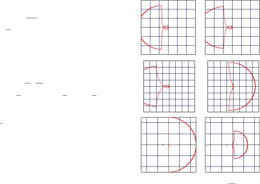
Figure 7.4 The (∞, 0)-Nyquist contour for RL(s) = s+1a , a = −2 (top left), a = −1 (top right), a = −12 (middle left), a = 12 (middle right), a = 1 (bottom left), and a = 2 (bottom right)

288	7 Frequency domain methods for stability		22/10/2004
		10
		5
	Im	0
		-5
		-10

-10	-5	0	5	10
		Re

Figure 7.5 The (∞, 0.1)-Nyquist contour for RL(s) = 1s

We can also check this directly by using Theorem 6.38. Since there are no unstable pole/zero cancellations in the interconnected system, IBIBO stability is determined by the zeros of the determinant, and the determinant is

	s + a + 1
1 + RL(s) =		.
	s + a

The zero of the determinant is −a − 1 which is in C− exactly when a > −1, and this is exactly the condition we derive above using the Nyquist criterion.

2.The previous example can be regarded as an implementation of a proportional controller.

Let’s give an integral controller a try. Thus we take RC (s) = 1s and RP (s) = s+1a . Once again, the conditions (i) and (ii) of Theorem 7.6 are satisfied, so we need only check condition (iii).

In this example the loop gain RL is strictly proper, and there is a pole of RL at s = 0. Thus we need to form a modified contour to take this into account. Let us expand the loop gain into its real and imaginary parts when evaluated on the imaginary axis away from the origin. We have

1					a
RL(iω) = −		− i					.
	ω2 + a2			ω(ω2 + a2)
Let us examine the image of {iω | ω > r} as r			becomes increasingly small. For ω near
				1
zero, the real part of the Nyquist contour is near −						, and as ω increases, it shrinks to
					ω2+a2

zero. Near ω = 0 the imaginary part is at −sgn(a)∞, and as ω increases, it goes to zero. Also note that the imaginary part does not change sign. The image of {iω | ω < −r} reflects this about the real axis. It only remains to examine the image of the contour r around s = 0 given by s = reiθ where θ [−π2 , π2 ]. The image of this contour under RL is

1 , θ [−π , π ]. reiθ(reiθ + a) 2 2

1 + RL(s) =

e−2iθ

22/10/2004

7.1 The Nyquist criterion

289

For su ciently small r we have

1

1

1

=

a

reiθ(reiθ + a)

reiθ

1 + r eiθ

a

=

1

1

1

r

eiθ +

reiθ a

· · ·

− a

iθ

=

e−

−

1

+ · · · .

ar

a2

Thus, as r → 0, the contour r gets mapped into a semi-circle of infinite radius, centred at a12 + i0, which goes clockwise from a12 + isgn(a)∞ to a12 − isgn(a)∞. In Figure 7.6 we

	10						10
	5						5
Im	0					Im	0
	-5						-5
	-10						-10
	-10	-5	0	5	10		-10	-5	0	5	10
			Re						Re
	10						10
	5						5
Im	0					Im	0
	-5						-5
	-10						-10
	-10	-5	0	5	10		-10	-5	0	5	10
			Re						Re
		Figure 7.6	The (∞, 0.1)-Nyquist contours for RL(s) =						1	, a =
									s(s+a)

−2 (top left), a = −1 (top right), a = 1 (bottom left), and a = 2 (bottom right)

plot the Nyquist contours.

Now we look at the particular case when a = 0. In this case RL(s) = s12 , and so the Nyquist contour is the image of the imaginary axis, except the origin, under RL, along

290

7 Frequency domain methods for stability

22/10/2004

with the image of the contour r as r → 0. On the imaginary axis we have RL(iω) = −ω12 . As ω goes from −∞ to 0− the Nyquist contour goes from 0− + i0 to −∞ + i0, and as ω goes from 0+ to +∞ the Nyquist contour goes from −∞ + i0 to 0− + i0. On the contourr we have

RL(reiθ) = r2 , θ [−π2 , π2 ].

As r → 0 this describes an infinite radius circle centred at the origin which starts at −∞ + i0 and goes around once in the clockwise direction. In particular, when a = 0 the Nyquist contour passes through the point −1 + i0. The contour is shown in Figure 7.7.

	100
	75
	50
	25
Im	0
	-25
	-50
	-75
	-75 -50 -25	0	25	50	75 100
		Re

Figure 7.7 The (∞, 0.1)-Nyquist contour for RL(s) = s12

We can now make the following conclusions regarding stability:

(a)when a < 0 the system is IBIBO unstable since np = 1 and there is one clockwise encirclement of the point −1 + i0;

(b)when a = 0 the system is IBIBO unstable since the Nyquist contour passes through the point −1 + i0;

(c)when a > 0 the system is IBIBO stable since np = 0 and there are no encirclements of the point −1 + i0.

We can also check IBIBO stability of the system via Theorem 6.38. Since there are no unstable pole/zero cancellations, we can look at the zeros of the determinant which is

s2 + as + 1 s2 + as .

By the Routh/Hurwitz criterion, the system is IBIBO stable exactly when a > 0, and this is what we ascertained using the Nyquist criterion.

3.Our final example combines the above two examples, and implements a PI controller

where we take RC (s) = 1 + 1s and RP (s) = s+1a . Here the condition (ii) of Theorem 7.6 holds, but we should examine (i) just a bit carefully before moving on. We have RL(s) =

s+1 1 , and so there is a pole/zero cancellation here when a = 1. However, it is a stable

s s+a

pole/zero cancellation, so condition (i) still holds. We also ascertain that RL has one pole in C+ when a < 0.

22/10/2004 7.1 The Nyquist criterion 291

In this example, RL is again strictly proper, and has a pole on the imaginary axis at the origin. Thus to compute the Nyquist contour we determine the image of the imaginary axis minus the origin, and tack on the image of the contour r = reiθ, θ [−π2 , π2 ]. We first compute

R	(iω) =	a − 1	−	i	ω2 + a	.
		ω2 + a2
L					ω(ω2 + a2)

Let’s first consider the situation when a 6= 0. In this case, as ω goes from −i∞ to 0−, the real part goes from 0 to aa−21 and the imaginary part goes from 0 to −sgn(a)∞. While the real part never changes sign, the imaginary part can change sign, so we must take care about how it is behaving. As ω goes from 0+ to +∞, the resulting part of the Nyquist contour is the mirror image about the real axis of what we have already computed. Now let us look at the image of the contour r. When a 6= 0 we have

reiθ

+ 1

1

RL(reiθ) =

a

reiθ

1 + r eiθ

a

· · ·

reiθ + 1

−

r

are

iθ

iθ

=

1

eiθ

+

iθ

a

1

e−

re

1

=

+

−

−

+ · · ·

a

ar

a2

a2

=e−iθ + a − 1 + · · ·

ar a2

From this we conclude that for a 6= 0 the image as r → 0 of r under RL is an infinite radius semi-circle centered at aa−21 and going clockwise from aa−21 + isgn(a)∞ to aa−21 − isgn(a)∞. In Figure 7.8 we show the Nyquist contours for various values of a 6= 0.

Now let us consider the image of the imaginary axis when a = 0. In this case we have

RL(iω) = −	1	− i	1	.
	ω2		ω

Thus the image of those points on the imaginary axis away from the origin describe a

parabola, sitting in C−, passing through the origin, and symmetric about the real axis. As concerns r when a = 0 we have

	e−iθ		e−iθ
RL(reiθ) = 1 +
	r		r

which, as r → 0, describes an infinite radius circle centred at the origin and going clockwise from −∞ + i0 to −∞ + i0. This Nyquist contour is shown in Figure 7.9. With the above computations and the corresponding Nyquist plots, we can make the following conclusions concerning IBIBO stability of the closed-loop system.

(a)For a < −1 the system is IBIBO unstable since np = 1 and there is one clockwise encirclement of −1 + i0.

(b)For a = −1 the system is IBIBO unstable since the Nyquist contour passes through the point −1 + i0.

(c)For −1 < a < 0 the system is IBIBO stable since np = 1 and there is one counterclockwise encirclement of the point −1 + i0.

(d)For a ≥ 0 the system is IBIBO stable since np = 0 and there are no encirclements of −1 + i0.

292		7	Frequency domain methods for stability									22/10/2004
	3							6
	2							4
	1							2
Im	0						Im	0
	-1							-2
	-2							-4
	-2	-1	0	1	2	3		-4	-2	0	2	4	6
			Re							Re
	10							10
	7.5							7.5
	5							5
	2.5							2.5
Im	0						Im	0
	-2.5							-2.5
	-5							-5
	-7.5							-7.5
	-7.5	-5 -2.5	0	2.5 5	7.5	10		-7.5	-5 -2.5	0	2.5 5	7.5	10
			Re							Re
	4							4
	2							2
Im	0						Im	0
	-2							-2
	-4							-4
	-4	-2	0	2	4			-4	-2	0	2	4
			Re							Re
		Figure 7.8								s+1	, a =
			The (∞, 0.2)-Nyquist contours for RL(s) = s(s+a)

−2 (top left), a = −1 (top right), a = −12 (middle left), a = 12 (middle right), a = 1 (bottom left), and a = 2 (bottom right)

22/10/2004

7.2 The relationship between the Nyquist contour and the Bode plot

293

30
20
10
Im	0
-10
-20
	-20	-10	0	10	20	30
			Re
Figure 7.9	The (∞, 0.2)-Nyquist contour for RL(s) = ss+12

As always, we can evaluate IBIBO stability with Theorem 6.38. To do this we can still simply look at the zeros of the determinant, because although there is a pole zero cancellation when a = 1, it is a cancellation of stable factors so it does not hurt us. We compute the determinant to be

	s2	+ (a + 1)s + 1
1 + RL(s) =				.
		s2
			+ as

An application of the Routh/Hurwitz criterion suggests that we have IBIBO stability for a > −1, just as we have demonstrated with the Nyquist criterion.

Note that the Nyquist criterion as we have shown is applicable only to interconnections with a simple structure, namely a single loop. Bode [1945] discusses a version of the Nyquist criterion for systems with multiple loops, and this is explored further by Zadeh and Desoer [1979]. However, the development is too significant, and the outcome too modest (what are obtained are su cient conditions for IBIBO stability under restrictive hypotheses) to make a presentation of these results worthwhile.

7.2 The relationship between the Nyquist contour and the Bode plot

The above examples, although simple, demonstrate that obtaining the Nyquist contour can be problematic, at least by hand. This is especially well illustrated by the third of the three examples where the capacity to change sign of the imaginary part of the restriction of RL to the imaginary axis causes some di culties which must be accounted for. A useful observation here is that the Nyquist contour is in essence the polar plot for the loop gain, taking care of the possibility of poles on the imaginary axis. The matter of constructing a Bode plot is often an easier one than that of building the corresponding polar plot, so a plausible approach for making a Nyquist contour is to first make a Bode plot, and convert this to a polar plot as discussed in Section 4.3.3.

7.2.1 Capturing the essential features of the Nyquist contour from the Bode plot

Let us illustrate this with the third of our examples from the previous section.

	294	7 Frequency domain methods for stability		22/10/2004
	7.9 Example (Example 7.8–3 cont’d) The loop gain, recall, is RL(s) =		s+1	. Let us write
			s(s+a)

this transfer function in the recommended form for making Bode plots. For a 6= 0 we have

1 1						1
RL(s) =							(s + 1).
	a		s		s	+ 1
					a

Thus the frequency response for RL is a product of four terms:

1			H2(ω) = −	i			1
H1(ω) =		,			,	H3(ω) =		, H4(ω) = 1 + iω.
	a			ω			1 + iωa

Each of these is a simple enough function for the purpose of plotting frequency response, and the e ect of a is essentially captured in H3.

Let us see if from Bode plot considerations we can infer when the imaginary part of the transfer function changes sign as ω goes from 0+ to +∞. In Example 7.8–3 we determined that as we vary ω in this way, the real part of the frequency response goes from aa−21 to 0 and the imaginary part goes from sgn(a)∞ to 0. The question is, “For which values of a does the imaginary part of the frequency response change sign as ω goes from 0+ to +∞?” Provided aa−21 < 0 this will happen if and only if the phase is ±π at some finite frequency ω¯. Let’s take a look at the phase of the frequency response function.

1.First we take a < 0. Since ]H1(ω) = π and ]H2(ω) = −π2 , in order to have the total phase equal ±π, it must be the case that

]H3(¯ω) + ]H4(¯ω) {π2 , −32π }.

The phase of H4 varies from 0 to π2 , and the phase of H3 varies from 0 to π2 (because a < 0!) Therefore we should aim for conditions on when ]H3(¯ω) + ]H4(¯ω) = π2 for some finite frequency ω¯. But one easily sees that for any a < 0 there will always be a finite frequency ω¯ so that this condition is satisfied since

lim ]H3(ω) + ]H4(ω) = π.

ω→∞

Thus as long as a < 0 there will always be a sign change in the imaginary part of the frequency response as we vary ω from 0+ to +∞. The Bode plots for RL are shown in Figure 7.10 for various a < 0.

2.Now we consider when a > 0. In this case we have ]H1(ω) = 0 and so we must seek ω¯ so that

]H3(¯ω) + ]H4(¯ω) {−π2 , 32π }.

However, since a > 0 the phase of H3 will go from 0 to −π2 . Therefore it will not be possible for ]H3(ω) + ]H4(ω) to equal either −π2 or 32π , and so we conclude that for a > 0 the imaginary part of RL(iω) will not change sign as we vary ω from 0+ to +∞. The Bode plots for RL are shown in Figure 7.11 for various a > 0.

7.2.2 Stability margins The above example illustrates how the Bode plot can be useful in determining certain aspects of the behaviour of the Nyquist contour. Indeed, if one gives this a short moments’ thought, one reaches the realisation that one can benefit a great deal by looking at the Bode plot for the loop gain. Let us provide the proper nomenclature for organising such observations.

22/10/2004

7.2 The relationship between the Nyquist contour and the Bode plot

295

	30
	20
	10
dB	0
	-10
	-20
	-30
	-40	-1	-0.5	0	0.5	1	1.5	2
	-1.5

log ω

	40
	20
dB	0
	-20
	-40	-1	-0.5	0	0.5	1	1.5	2
	-1.5

log ω

	150									150
	100									100
deg	50								deg	50
	0									0
	-50									-50
	-100									-100
	-150									-150
	-1.5	-1	-0.5	0	0.5	1	1.5	2		-1.5	-1	-0.5	0	0.5	1	1.5	2

log ω

log ω

	40
	20
dB	0
	-20
	-40	-1	-0.5	0	0.5	1	1.5	2
	-1.5

log ω

	150
	100
deg	50
	0
	-50
	-100
	-150
	-1.5	-1	-0.5	0	0.5	1	1.5	2

log ω

Figure 7.10 Bode plots for RL(s) =	s+1		for a = −2 (top left),
	s(s+a)

a = −1 (top right), and a = −12 (bottom)

7.10 Definition Let RL R(s) be a proper rational function forming the loop gain for the interconnection of Figure 7.12. Assume that there is no frequency ω > 0 for which RL(iω) = −1 + i0.

(i)A phase crossover frequency, ωpc [0, ∞), for RL is a frequency for which ]RL(iωpc) = 180◦.

Let ωpc,1, . . . , ωpc,` be the phase crossover frequencies for RL, and assume these are ordered so that

RL(iωpc,1) < · · · < RL(iωpc,`).

Also suppose that for some k {1, . . . , `} we have

RL(iωpc,k) < −1 < RL(iωpc,k + 1).

296

7 Frequency domain methods for stability

22/10/2004

	40
	20
dB	0
	-20
	-40	-1	-0.5	0	0.5	1	1.5	2
	-1.5

log ω

	40
	20
dB	0
	-20
	-40	-1	-0.5	0	0.5	1	1.5	2
	-1.5

log ω

	150								150
	100								100
deg	50							deg	50
	0								0
	-50								-50
	-100								-100
	-150								-150
	-1.5	-1	-0.5	0	0.5	1	1.5	2

log ω

-1.5 -1 -0.5 0 0.5 1 1.5 2 log ω

	30
	20
	10
dB	0
	-10
	-20
	-30
	-40	-1	-0.5	0	0.5	1	1.5	2
	-1.5

log ω

	150
	100
deg	50
	0
	-50
	-100
	-150
	-1.5	-1	-0.5	0	0.5	1	1.5	2

log ω

Figure 7.11 Bode plots for RL(s) =	s+1		for a =	1	(top left),
	s(s+a)			2

a = 1 (top right), and a = 2 (bottom)

rˆ(s) RL(s) yˆ(s)

−

Figure 7.12 Unity gain feedback loop for stability margin discussion

22/10/2004

7.2 The relationship between the Nyquist contour and the Bode plot

297

(ii) The lower gain margin for RL defined by

Kmin = −RL(iωpc,k)−1 (0, 1).

If

−1 < RL(iωpc,1) < · · · < RL(iωpc,`),

then Kmin is undefined.

(iii) The upper gain margin for RL is defined by

Kmax = −RL(iωpc,k + 1)−1 (1, ∞).

If

RL(iωpc,1) < · · · < RL(iωpc,`) < −1,

then Kmax is undefined.

(iv) A gain crossover frequency, ωgc [0, ∞), for RL is a frequency for which |RL(iωgc)| = 1.

Let ωgc,1, . . . , ωgc,` be the gain crossover frequencies for RL, and assume these are ordered so that

](RL(iωgc,1)) < · · · < ](RL(iωgc,`)).

(v) The lower phase margin for RL is defined by

Φ		=	180◦ − ](RL(iωgc,`)),	](RL(iωgc,`)) ≥ 0
	min		(undefined,	](RL(iωgc,`)) < 0.

(vi) The upper phase margin for RL is defined by

Φ		=	](RL(iωgc,1)) + 180◦,	](RL(iωgc,1)) ≤ 0
	max		(undefined,	](RL(iωgc,1)) > 0.

Let us parse these definitions, as they are in actuality quite simple. First of all, we note that it is possible to read the gain and phase margins o the Nyquist plot; this saves one having to compute them directly using the definitions. Rather than try to state in a precise way how to procure the margins from the Nyquist plot, let us simply illustrate the process in Figure 7.13. The basic idea is that for the gain margins, one looks for the positive frequency crossings of the negative real axis closest to −1 + i0 in each direction. The reciprocal of the distances to the imaginary axis are the gain margins, as indicated in Figure 7.13. For the phase margins, one looks for the positive frequency crossings of the unit circle closest to the point −1 + i0. The angles to the negative real axis are then the phase margins, again as indicated in Figure 7.13. We shall adopt the convention that when we simply say phase margin, we refer to the smaller of the upper and lower phase margins.

The interpretations of gain crossover and phase crossover frequencies are clear. At a gain crossover frequency, the magnitude on the Bode plot for RL will be 0dB. At a phase crossover frequency, the graph will cross the upper or lower edge of the phase Bode plot. Note that it is possible that for a given loop gain, some of the margins may not be defined. Let us illustrate this with some examples.

298	7 Frequency domain methods for stability	22/10/2004
	Im	Im
	−1 + i0
	Re
K−1	K−1
min	max
	Φmin	1
		Re
	Φmax

Figure 7.13 Getting gain (left) and phase (right) margins from the

	Nyquist plot
3		10
		0
		-10
2	dB	-20
		-30
		-40
1		-50
		-1.5	-1	-0.5	0	0.5	1	1.5	2

log ω

Im	0

						150
-1						100
						50
					deg
						0
-2						-50
						-100
						-150
-1	0	1	2	3	4	-1.5	-1	-0.5	0	0.5	1	1.5	2
								log ω
			Re

Figure 7.14 Nyquist and Bode plots for RL(s) =	10
	s2+4s+3

7.11 Examples 1. We consider the loop gain

10

RL(s) = s2 + 4s + 3.

In Figure 7.14 we note that there is one gain crossover frequency, and it is roughly at ωgc = 2.1. The phase at the gain crossover frequency is about −110◦, which gives the upper phase margin as Φmax ≈ 70◦. The lower phase margin is not defined. Also, neither of the gain margins are defined.

2. We take as loop gain

10

RL(s) = −s2 + 4s + 3.

The Bode and Nyquist plots are shown in Figure 7.15. From the Bode plot we see that there is one gain crossover frequency and it is approximately at ωgc = 2.1. The phase at the gain crossover frequency it is about 70◦. Thus the lower phase margin is