08.Performance of control systems

This version: 22/10/2004

Chapter 8

Performance of control systems

Before we move on to controller design for closed-loop systems, we should carefully investigate to what sort of specifications we should make our design. These appear in various ways, depending on whether we are working with the time-domain, the s-domain, or the frequency-domain. Also, the interplay of performance and stability can be somewhat subtle, and there is often a tradeo to be made in this regard. Our objective in this chapter is to get the reader familiar with some of the issues that come up when discussing matters of performance. Also, we wish to begin the process of familiarising the reader with the ways in which various system properties can a ect the performance measures. In many cases, intuition is one’s best friend when such matters come up. Therefore, we take a somewhat intuitive approach in Section 8.2. The objective is to look at tweaking parameters in a couple of simple transfer function to see how they a ect the various performance measures. It is hoped that this will give a little insight into how one might, say, glean some things about the step response by looking at the Bode plot. The matter of tracking and steady-state error can be dealt with in a more structured way. Disturbance rejection follows along similar lines. The final matter touched upon in this chapter is the rˆole of the sensitivity function in the performance of a unity gain feedback loop. The minimisation of the sensitivity function is often an objective of a successful control design, and in the last section of this chapter we try to indicate why this might be the case.

Contents

8.1	Time-domain performance specifications . . . . . . . . . . . . . . . . . . . . . . . . . . . .		318
8.2	Performance for some classes of transfer functions . . . . . . . . . . . . . . . . . . . . . .		320
	8.2.1	Simple first-order systems . . . . . . . . . . . . . . . . . . . . . . . . . . . . . . . .	320
	8.2.2	Simple second-order systems . . . . . . . . . . . . . . . . . . . . . . . . . . . . . .	321
	8.2.3 The addition of zeros and more poles to second-order systems . . . . . . . . . . .		326
	8.2.4	Summary . . . . . . . . . . . . . . . . . . . . . . . . . . . . . . . . . . . . . . . . .	327
8.3	Steady-state error . . . . . . . . . . . . . . . . . . . . . . . . . . . . . . . . . . . . . . . .		328
	8.3.1 System type for SISO linear system in input/output form . . . . . . . . . . . . . .		329
	8.3.2 System type for unity feedback closed-loop systems . . . . . . . . . . . . . . . . .		333
	8.3.3	Error indices . . . . . . . . . . . . . . . . . . . . . . . . . . . . . . . . . . . . . . .	336
	8.3.4 The internal model principle . . . . . . . . . . . . . . . . . . . . . . . . . . . . . .		336
8.4	Disturbance rejection . . . . . . . . . . . . . . . . . . . . . . . . . . . . . . . . . . . . . .		336
8.5	The sensitivity function . . . . . . . . . . . . . . . . . . . . . . . . . . . . . . . . . . . . .		342

318		8 Performance of control systems	22/10/2004
	8.5.1 Basic properties of the sensitivity function . . . . . . . . . . . . . . . .		. . . . . . 343
	8.5.2	Quantitative performance measures . . . . . . . . . . . . . . . . . . . .	. . . . . . 344
8.6	Frequency-domain performance specifications . . . . . . . . . . . . . . . . . . .		. . . . . . 346
	8.6.1	Natural frequency-domain specifications . . . . . . . . . . . . . . . . . .	. . . . . . 346
	8.6.2 Turning time-domain specifications into frequency-domain specifications		. . . . . 350
8.7	Summary . . . . . . . . . . . . . . . . . . . . . . . . . . . . . . . . . . . . . . .		. . . . . . 350

8.1 Time-domain performance specifications

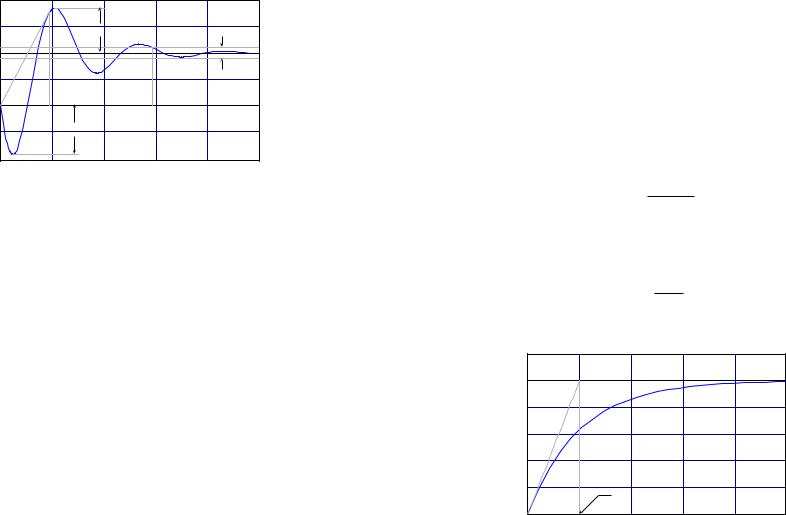
We begin with describing what is a common manner for specifying the desired behaviour of a control system. The idea is essentially that the system is to be given a step input, and the response is to have various specified properties. You will recall in Proposition 3.40, it was shown how to determine the step response by solving an initial value problem. In this chapter we will be producing many step responses, and in doing so we have used this initial value problem method. In any case, when one gives a BIBO stable input/output system a step input, it will, after some period of transient response, settle down to some steady-state value. With this in mind, we make some definitions.

8.1 Definition Let (N, D) be a BIBO stable SISO linear system in input/output form, let 1N,D(t) be the step response, and suppose that limt→∞ 1N,D(t) = 1ss R. (N, D) is step-

pable provided that 1ss 6= 0.	For a steppable system (N, D), let y(t) be the response to
the reference r(t) = 1(t)(1ss)−1	so that limt→∞ y(t) = 1. We call y(t) the normalised step
response.
(i) The rise time is defined by								≤ δ
tr	=		δ		δ		y(t)
		sup						t for all t		[0, δ] .
(ii) For (0, 1) the -settling time is defined by
ts, =	δ		δ		|y(t) − 1| < for all t [δ, ∞) .
	inf

(iii)The maximum overshoot is defined by yos = supt{y(t) − 1} and the maximum percentage overshoot is defined by Pos = yos × 100%.

(iv)The maximum undershoot is defined by yus = supt{−y(t)} and the maximum

percentage undershoot is defined by Pus = yus × 100%.

For the most part, these definitions are self-explanatory once you parse the symbolism. A possible exception is the definition of the rise time. The definition we provide is not the usual one. The idea is that rise time measures how quickly the system reaches its steady-state value. A more intuitive way to measure rise time would be to record the smallest time at which the output reaches a certain percentage (say 90%) of its steady-state value. However, the definition we provide still gives a measure of the time to reach the steady-state value, and has the advantage of allowing us to state some useful results. In any event, a typical step response is shown in Figure 8.1 with the relevant quantities labelled.

Notice that in Definition 8.1 we introduce the notion of a steppable input/output system. The following result gives an easy test for when a system is steppable.

22/10/2004

8.1 Time-domain performance specifications

319

yos	2²
y(t)
tr	ts,²
yus
	t

Figure 8.1 Performance parameters in the time-domain

8.2 Proposition A BIBO stable SISO linear system (N, D) in input/output form is steppable if and only if lims→0 TN,D(s) 6= 0. Furthermore, in this case limt→∞ 1N,D(t) = TN,D(0).

Proof By the Final Value Theorem, Proposition E.9(ii), the limiting value for the step response is

		ˆ	(s).
lim 1N,D(t) = lim s1N,D(s) = lim TN,D
t→∞	s→0	s→0
		ˆ
Therefore limt→∞ 1N,D(t) 6= 0 if and only if lims→0 1N,D(s) 6= 0, as specified.

So it is quite simple to identify systems which are not steppable. The idea here is quite simple. When lims→0 TN,D(s) = 0 this means that the input only appears in the di erential equation after being di erentiated at least once. For a step input, this means that the righthand side of the di erential equation forming the initial value problem is zero, and since (N, D) is BIBO stable, the response must decay to zero. The following examples illustrate both sides of the story.

8.3Examples 1. We first take (N(s), D(s)) = (1, s2 +2s+2). By Proposition 3.40 the initial value problem to solve for the step response is

¨ ˙

1N,D(t) + 2 1N,D(t) + 2 1N,D(t) = 1, y(0) = 0, y˙(0) = 0.

The step response here is computed to be

1N,D(t) = 12 − 12 e−t(cos t + sin t).

Note that limt→∞ 1N,D(t) = 12 , and so the system is steppable. Therefore, we can compute the normalised step response, and it is

y(t) = 1 − e−t(cos t + sin t).

2.Next we take (N(s), D(s)) = (s, s2 + s2 + 2). Again by Proposition 3.40, the initial value problem to be solved is

¨ ˙

1N,D(t) + 2 1N,D(t) + 2 1N,D(t) = 0, y(0) = 0, y˙(0) = 1.

The solution is 1N,D(t) = e−t sin t which decays to zero, so the system is not steppable. This is consistent with Proposition 8.2 since lims→0 TN,D(s) = 0.

320

8 Performance of control systems

22/10/2004

8.2 Performance for some classes of transfer functions

It is quite natural to specify performance criteria in the time-domain. However, in order to perform design, one needs to see how system parameters a ect the time-domain performance, and how various performance measures get reflected in the other representations of control systems—the Laplace transform domain and the frequency-domain. To get a feel for this, in this section we look at some concrete classes of transfer functions.

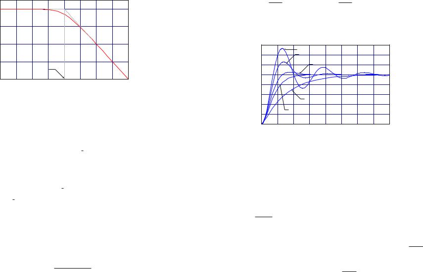
8.2.1 Simple first-order systems The issues surrounding performance of control systems can be di cult to grasp, so our approach will be to begin at the beginning, describing what happens with simple systems, then moving on to talk about things more general. In this, the first of the three sections devoted to rather specific transfer functions, we will be considering the situation when the transfer function

TL(s) =

RL(s)

1 + RL(s)

has a certain form, without giving consideration to the precise form of the loop gain RL. The simplest case one can deal with is one where the system transfer function is first order. If we normalise the transfer function so that it will have a steady-state response of 1 to a unit step input, the transfer functions under consideration look like

1

Tτ (s) = τs + 1,

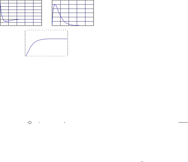
and so essentially depend upon a single parameter τ. The step response of such a system is depicted in Figure 8.2. The parameter τ is exactly the rise time for a first-order system, at

y(t)

t = τ

t

Figure 8.2 Step-response for typical first-order system

least by our definition of rise time. Thus, by making τ smaller, we ensure the system will more quickly reach its steady-state value.

Let’s see how this is reflected in the behaviour of the poles of the transfer function, and in the Bode plot for the transfer function. The behaviour of the poles in this simple first-order case is straightforward. There is one pole at s = −τ1 . Thus making τ smaller moves this

22/10/2004

8.2 Performance for some classes of transfer functions

321

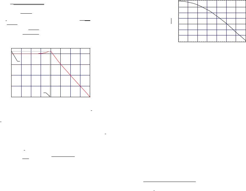
pole further from the origin, and further into the negative complex plane. Thus the issues in designing a first-order transfer function are one: move the pole as far to the left as possible. Of course, not many transfer functions that one will obtain are first-order.

The Bode plot for the transfer function Tτ is very simple, of course: it has a single break frequency at ω = τ1 . A typical such plot is shown in Figure 8.3. Obviously, the greater

dB
ω =	1
	τ

log ω

Figure 8.3 Bode plot for typical first-order system

values of break frequency correspond to quicker response times. Thus, for simple first-order systems, the name of the game can be seen as pushing the break frequency as far as possible to the right. This is, in fact, a general strategy, and we begin an exploration of this by stating an obvious result.

8.4 Proposition The magnitude of Tτ (s) at s =					i		1
						is	√2 .
					τ
Proof This is a simple calculation since
Tτ	i		=			1	,
	τ			i + 1
			1
whose magnitude we readily compute to be			√2 .
1								i
We also compute 20 log √2 ≈ −3.01dB. Thus the magnitude of Tτ (									) is approximately −3dB
								τ

which one can easily pick o from a Bode plot. We call τ1 the bandwidth for the first-order transfer function. Note that for first-order systems, larger bandwidth translates to better performance, at least in terms of rise time.

8.2.2 Simple second-order systems First-order systems are not capable of sustaining much rich behaviour, so let’s see how second-order systems look. After again requiring a transfer function which produces a steady-state of 1 to a unit step input, the typical secondorder transfer function we look at is

ω2

Tζ,ω0 (s) = s2 + 2ζω00s + ω02 ,

322 8 Performance of control systems 22/10/2004

which depends on the parameters ζ and ω0. If we are interested in BIBO stable transfer functions, the Routh/Hurwitz criterion, and Example 5.35 in particular, then we can without loss of generality suppose that both ζ and ω0 are positive.

The nature of the closed form expression for the step response depends on the value of ζ. In any case, using Proposition 3.40(ii), we ascertain that the step response is given by

1 + ω√0t

− 1 e(−ζ−√

√

ζ

e(−ζ+√

ζ

ζ2−1)ω0t −

ζ2−1)ω0t, ζ > 1

y(t) =

ζ2−1

ζ2−1

1

−

e (1 + ω0t),

ζ = 1

ζω0t

2

ζ

2

cos(p

ω0t) , ζ < 1.

1 − e−

1 − ζ

ω0t) + √1−ζ2 sin(p

1 − ζ

This is plotted in Figure 8.4 for various values

of ζ

.

Note that for large ζ there is no

ζ = 0.2

ζ = 0.4

ζ = 0.7

y(t)

ζ = 2

ζ = 1

t

Figure 8.4 Step response for typical second-order system for various values of ζ

overshoot, but that as ζ decreases, the response develops an overshoot. Let us make some precise statements about the character of the step response of a second-order system.

8.5 Proposition Let y(t) be the step response for the SISO linear system (N, D) with transfer function Tζ,ω0 . The following statements hold:

(i)	when ζ ≥ 1 there is no overshoot;
	when ζ < 1 there is overshoot, and it has magnitude yos = e−πζ/√						and occurs at
(ii)						1−ζ2
		√	π
	time tos =			ω0	;
(iii)			1−ζ2
	if ζ < 1 the rise time satisfies

p		p		p		e−p0
							r trp1 − ζ2.
− (eω0ζtr	1 − ζ2) +		1 − ζ2 cos(ω0		1 − ζ2tr) + (ω0tr + ζ) sin(ω0		1 − ζ2tr) =

ω ζt

Proof (i) and (ii) The proof here consists of di erentiating the step response and setting it to zero to obtain those times at which it is zero. When ζ ≥ 1 the derivative is zero only when

p

t = 0. When ζ < 1 the derivative is zero when ω0 1 − ζ2t = nπ, n Z+. The smallest

22/10/2004

8.2 Performance for some classes of transfer functions

323

positive time will be the time of maximum overshoot, so we take n = 1, and from this the stated formulae follow.

(iii) The rise time tr is the smallest positive time which satisfies

y˙(t0) = y(t0), t0

since the slope at the rise time should equal the slope of the line through the points (0, 0) and (t0, y(t0)). After some manipulation this relation has the form stated in the proposition.

In Figure 8.5 we plot the maximum overshoot and the time at which it occurs as a function of

1					40
					35
0.8					30
0.6					25
				0
os				ω	20
				os
y				t
0.4					15
					10
0.2
					5
0.2	0.4	0.6	0.8	1
		ζ

0.2	0.4	0.6	0.8	1
		ζ

Figure 8.5 Maximum overshoot (left) and time of maximum overshoot (right) as functions of ζ

ζ. Note that the overshoot decreases as ζ increases, and that the time of overshoot increases as ζ increases.

The rise time tr is not easily understood via an analytical formula. Nevertheless, we may numerically determine the rise time for various ζ and ω0 by solving the equation in part (iii) of Proposition 8.5 and the results are shown in Figure 8.6. In that same figure we also plot the

curve tr = 5ω90 , and we see that it is a very good approximation—indeed it is indistinguishable in our plot from the curve for ζ = 0.9. Thus, for second-order transfer functions Tζ,ω0 (s) with

ζ< 1, it is fair to use tr ≈ 9ω50 . Of course, for more general transfer functions, even more general second-order transfer functions (say, with nontrivial numerators), this relationship can no longer be expected to hold.

From the above discussion we see that overshoot is controlled by the damping factor ζ and rise time is essentially controlled by the natural frequency ω0. However, we note that the time for maximum overshoot, tos, depends only upon ζ, and indeed increases as ζ increases. Thus, there is a possible tradeo to make when selecting ζ if one chooses a small in the

-settling time specification. A commonly used rule of thumb is that one should choose
1	which leads to yos = e−	π	≈ 0.043 and tosω0	= π	√
ζ = √2					2 ≈ 4.44.

Let’s look now to see how the poles of Tζ,ω0 depend upon the parameters ζ and ω0. One

p

readily determines that the poles are ω0(−ζ ± 1 − ζ2). As we have just seen, good response

324

8 Performance of control systems

22/10/2004

25
20
15	ζ = 0.1
r
t	ζ = 0.5
10
5
ζ = 0.9 and		9
		5ω0
0.25	0.5	0.75	1	1.25	1.5	1.75	2
			ω0

Figure 8.6 Behaviour of rise time versus ω0 for various ζ < 1

dictates that we should have poles with nonzero imaginary part, so we consider the situation when ζ < 1. In this case, the poles are located as in Figure 8.7. Thus the poles lie on a circle

θ	p1 − ζ 2ω0
ω0
Im
−ζω0
ω0
θ
	Re

Figure 8.7 Pole locations for Tζ,ω0 when 0 < ζ < 1

of radius ω0, and the angle they make with the imaginary axis is sin−1 ζ. Our rule of thumb

of taking ζ = 1 then specifies that the poles lie on the rays emanating from the origin into

√

2

C− at an angle of 45◦ from the imaginary axis.

Finally, for second-order systems, let’s see how the parameters ζ and ω0 a ect the Bode plot for the system. In Exercise E4.6 the essential character of the frequency response for Tζ,ω0 is investigated, and let us just record the outcome of this.

8.6 Proposition If Hζ,ω0 (ω) = Tζ,ω0 (iω), then the following statements hold:

22/10/2004

8.2 Performance for some classes of transfer functions

325

326

8 Performance of control systems

22/10/2004

(i)

|Hζ,ω0 (ω)| =

p

ω02

;

2.4

(ω2

ω2)2 + 4ζ

2ω2

ω2

2.2

(ii)

H

0 − 2ζω0

ω

;

0

2

]

ζ,ω0

(ω) = arctan

−

√2

ω02 − ω2

0

|

2ζ

√1 ζ2

0

1.8

(iii)

7→ |

at the frequency

ω

ω

for ζ < 1 , the function ω

Hζ,ω (ω) has a maximum of

1

−

ζ,ω

0

ωm = ω0p1 − 2ζ2;

1.6

1

2ζ2

1.4

(iv)

]Hζ,ω0 (ωm) = arctan −p

ζ−

.

1.2

In Figure 8.8 we label the typical points on the Bode plot for the transfer function Tζ,ω0

1

0.1

0.2

0.3

0.4

0.5

0.6

0.7

ζ

Figure 8.9 Dependence of bandwidth on ζ for second-order sys-

|Hζ,ω0 (ωm)|

tems

dB

8.2.3 The addition of zeros and more poles to second-order systems

In our general

buildup, the next thing we look at is the e ect of adding to a second-order transfer function

either a zero, i.e., making a numerator which has a root, or an additional pole. The idea is

that we will investigate the e ect that these have on the nature of the second-order response.

detail

This is carried out by Jr. [1949].

ωm

Adding a zero To investigate what happens to the time signal when we add a zero to a

log ω

second-order system with a zero placed at −αζω0. If we normalise the transfer function to

that it has unit value at s = 0, we get

Figure 8.8 Typical Bode plot for second-order system with ζ < 1

√

2

when ζ < 1 . As we decrease ζ the peak becomes larger, and shifted to the left. The phase,

√

2

as we decrease ζ, tends to −90◦ at the peak frequency ωm.

Based on the discussion with first-order systems, for a second-order system with transfer

function Tζ,ω0 , the bandwidth is that frequency ωζ,ω0 > 0 for which |Tζ,ω0 (iωζ,ω0 )| = 12 . The

√

following result gives an explicit expression for bandwidth of second-order transfer functions. Its proof is via direct calculation.

8.7 Proposition When ζ < 1 the bandwidth for Tζ,ω satisfies

√2 0

ωζ,ω0 = 1 − 2ζ2 + p2(1 − 2ζ2) + 4ζ4. ω0

Thus we see that the bandwidth is directly proportional to the natural frequency ω0. The dependence on ζ is shown in Figure 8.9. Thus we duplicate our observation for first-order systems that one should maximise the bandwidth to minimise the rise time. This is one of the general themes in control synthesis, namely that, all other things being constant, one should maximise bandwidth.

	ω2		s + αζω	0
T (s) =	0				.
	αζω0		s2 + 2ζω0s + ω02

For concreteness we take ζ = 12 and ω0 = 1. The step responses and magnitude Bode plots are shown in Figure 8.10 for various values of α. We note a couple of things.

8.8Remarks 1. The addition of a zero increases the overshoot for α < 3, and dramatically so for α < 1.

2.If the added zero is nonminimum phase, i.e., when α < 0, the step response exhibits undershoot. Thus nonminimum phase systems have this property of reacting in a manner contrary to what we want, at least initially. This phenomenon will be explored further in Section 9.1.

3.The magnitude Bode plot is the same for α = −12 as it is for α = 12 . Where the Bode plots will di er is in the phase, as in the former case, the system is nonminimum phase.

4.When comparing the step response and the magnitude Bode plots for positive α’s, one

sees that the general tendency of larger bandwidths1 to produce shorter rise times is preserved.

1We have not yet defined bandwidth for general transfer functions, although it is clear how to do so. The bandwidth, roughly, is the smallest frequency above which the magnitude of the frequency response remains

below 1 times its zero frequency value. This is made precise in Definition 8.25.

√

2

22/10/2004

8.2 Performance for some classes of transfer functions

327

	3
		α = 0.5
		α = 1
	2	α = 2
PSF1Sigma(t)	1
		α = 0
	0
	-1	α = −0.5
	2	4	6	8	10	12	14
				PSFt
	0
-20		α = ±21
dB -40				α = 1
					α = 2

-60

α = 0

-80

-1.5 -1 -0.5

0

0.5

1

1.5

2

log ω

Figure 8.10 The e ect of an added zero for α = −12 , 0, 12 , 1, 2

Adding a pole Now we look at the e ect of an additional pole at −αζω0. The normalised transfer function is

	αζω03
T (s) =		.
	(s + αζω0)(s2 + 2ζω0s + ω02)

We once again fix ζ = 12 and ω0 = 1, and plot the step response for varying α in Figure 8.11. We make the following observations.

8.9 Remarks 1. If a pole is added with α < 3, the rise time will be dramatically increased. This is also reflected in the bandwidth of the system increasing with α.

2.The larger bandwidths in this case are accompanied by a more pronounced peak in the Bode plot. As with second-order systems where this is a consequence of a smaller

damping factor, we see that there is more overshoot.

8.2.4 Summary This section has been something of a mixed bag of examples and informal observations. We do not try to make it more than that at this point. Some of the things covered here have a more general and rigorous treatment in Chapter 9. However, it is worth summarising the gist of what we have said in an informal way. These are not theorems. . .

1. Increased bandwidth can mean shorter rise times.

328

8 Performance of control systems

22/10/2004

		α = 10
	1.2
PSF1Sigma(t)	1 α = 2
	0.8
	0.6			α = 0.5
	0.4
			α = 1
	0.2
	2	4	6	8	10	12	14
				PSFt

	0
	-20
							α
	-40
dB	-60
	-80
	-100
	-120
	-1.5	-1	-0.5	0	0.5	1	1.5	2

log ω

Figure 8.11 The e ect of an added pole for α = 12 , 1, 2, 10

2.In terms of poles, larger bandwidth sometimes means closed-loop poles that are far from the imaginary axis.

3.Large overshoot can arise when the Bode plot exhibits a large “peak” at some frequency. This is readily seen for second-order systems, but can happen for other systems.

4.In terms of poles of the closed-loop transfer function, large overshoot can arise when poles are close to the imaginary axis, as compared to their distance from the real axis.

5.Zeros of the closed-loop transfer function lying in C+ can lead to undershoot in the step response, this having a deleterious e ect on the system’s performance.

These rough guidelines can be useful in predicting the behaviour of a system based upon the location of its poles, or on the shape of its frequency response. The former connection forms the basis for root-locus design which is covered in Chapter 11. The frequency response ideas we shall make much use of, as they form the basis for the design methodology of Chapters 12 and 15. It is existence of the rigorous mathematical ideas for control design in Chapter 15 that motivate the use of frequency response methods in design.

8.3 Steady-state error

An important consideration is that the di erence between the reference signal and the output should be as small a possible. When we studied the PID controller in Section 6.5

22/10/2004

8.3 Steady-state error

329

we noticed that with an integrator it was possible to make at least certain types of transfer function have no steady-state error. Here we look at this in a slightly more systematic manner. The first few subsections deal with descriptive matters.

8.3.1 System type for SISO linear system in input/output form For a SISO system (N, D) in input/output form, a controlled output is a pair (r(t), y(t)) defined for t [0, ∞) with the property that

D ddt y(t) = N ddt r(t)

The error for a controlled output (r(t), y(t)) is e(t) = r(t) − y(t), and the steady-state error is

lim (r(t) − y(t)),

t→∞

and we allow the possibility that this limit may not exist. With this language, we have the following definition of system “type.”

8.10 Definition Let k ≥ 0. A signal r U defined on [0, ∞) is of type k if r(t) = Ctk for some C > 0. A BIBO stable SISO linear system (N, D) is of type k if limt→∞(r(t) − y(t)) exists and is nonzero for every controlled output (r(t), y(t)) with r(t) of type k.

In the definition of the type of a SISO linear system in input/output form, it is essential that the system be BIBO stable, i.e., that the roots of D all lie in C−. If this is not the case, then one might expect the output to grow exponentially, and so error bounds like those in the definition are not possible.

The following result attempts to flush out all the implications of system type.

8.11 Proposition Let (N, D) be a BIBO stable SISO linear system in input/output form. The following statements are equivalent:

(i) (N, D) is of type k;

(ii)	limt→∞(r(t) − y(t)) exists and is nonzero for some controlled output (r(t), y(t)) with
	r(t) of type k.
The		1
(iii)	lim		1 − TN,D(s)	exists and is nonzero.
	s→0	sk
	preceding three equivalent statements imply the following:
(iv)	limt→∞(r(t) − y(t)) = 0 for every controlled output (r(t), y(t)) with r(t) of type ` with
	` < k.

Proof (i) (ii) That (i) implies (ii) is clear. To show the converse, suppose that limt→∞(¯r(t) − y¯(t)) = K for some nonzero K and for some controlled output (¯r(t), y¯(t))

with r¯(t) of type k.

Suppose that deg(D) = n and let y1(t), . . . , yn(t) be the n linearly

independent solutions to D

d

y(t) = 0. If y¯ (t) is a particular solution to D

d

y(t) = r¯(t)

dt

we must have

p

dt

y¯(t) = c¯1y1(t) + · · · + c¯nyn(t) + y¯p(t)

for some c¯1, . . . , c¯n R. By hypothesis we then have

t→∞ r¯(t) − y¯p(t)

t→∞

−

1 1

(t)

− · · · −

n

n

(t)

−

p

= K.

lim r¯(t)

c¯ y

c¯ y

y¯ (t)

= lim

Here we have used the fact that the roots of D are in C− so the solutions y1(t), . . . , yn(t) all decay to zero.

330

8 Performance of control systems

22/10/2004

Now let (r(t), y(t)) be a controlled output with r(t) be an arbitrary signal of type k. Note that we must have r(t) = Ar¯(t) for some A > 0. We may take yp(t) = Ay¯p(t) as a particular solution to D ddt y(t) = N ddt r(t) by linearity of the di erential equation. This means that we must have

y(t) = c1y1(t) + · · · + cnyn(t) + Ay¯p(t)

for some c1, . . . , cn R. Thus we have

tlim

r(t) − y(t) =

tlim

Ar¯(t) − c1y1(t) − · · · − cnyn(t) − Ay¯p(t)

→∞

=

→∞

A r¯(t)

−

lim

y¯ (t)

= AK.

t→∞

p

This completes this part of the proof.

with r(t) =

tk , and suppose that

(ii) (iii) Let (r(t), y(t)) be a controlled output

1

k!

y(0) = 0, y(1)(0) = 0 . . . , y(n−1)(0) = 0.

Note that rˆ(s) =

. Taking the Laplace trans-

sk+1

form of the di erential equation D

d

d

y(t) = N dt

r(t) gives D(s)ˆy(s) = N(s)ˆr(s). By

Proposition E.9(ii) we have

dt

tlim r(t) − y(t)

= lim s rˆ(s)

−

yˆ(s)

s→0

(s)ˆr(s)

→∞

= lim s rˆ(s)

−

T

s→0

N,D

1

T

N,D

(s)

−

= lim s

sk+1

s→0

from which we ascertain that

lim r(t)

y(t) = lim

1

TN,D(s)

.

(8.1)

−

− sk

t→∞

s→0

From this the result clearly follows. (iii) = (iv) Suppose that

1 − TN,D(s) = K sk

for some nonzero constant K and let ` {0, 1, . . . , k − 1}. Let (r(t), y(t)) be a controlled output with r(t) a signal of type `. Since the roots of D are in C−, we can without loss of generality suppose that y(0) = 0, y(1)(0) = 0, . . . , y(n−1)(0) = 0. We then have

lim r(t)		y(t)		lim	1			TN,D(s)
t→∞	−		=	s→0			−	1s`	TN,D(s)
			= lim sk−`					−	sk
				s→0
			= K lim sk−` = 0.
				s→0
This completes the proof.

Let us examine the consequences of this result by making a few observations.

8.12 Remarks 1. Although we state the definition for systems in input/output form, it obviously applies to SISO linear systems and to interconnected SISO linear systems since these give rise to systems in input/output form after simplification of their transfer functions.

22/10/2004

8.3 Steady-state error

331

2.The idea is that a system of type k can track up to a constant error a reference signal which is a polynomial of degree k. Thus, for example, a system of type 0 can track a step input up to a constant error. A system of type 1 can track a ramp input up to a

constant error, and can exactly track a step input for large time.

Let’s see how this plays out for some examples.

8.13 Examples In each of these examples we look at a transfer function, decide what is its type, and plot its response to inputs of various types.

1. We take

1 TN,D(s) = s2 + 3s + 2.

This transfer function is type 0, as may be determine by checking the limit of part (iii) of Proposition 8.11. For a step reference, ramp reference, and parabolic reference,

r		(t) =	1,	t ≥ 0
1			(0,	otherwise
r		(t) =	t,	t ≥ 0
2			(0,	otherwise
3			(0,	otherwise,
r	(t) =		t2,	t ≥ 0

respectively, we may ascertain using Proposition 3.40, that the step, ramp, and parabolic responses are

y1(t) = 12 + 12 e−2t − e−t, y2(t) = 14 (2t − 3) − 14 e−2t + e−t, y3(t) = 14 (2t2 − 6t + 7) + 14 e−2t − 2e−t,

and the errors, ei(t) = ri(t) − yi(t), i = 1, 2, 3, are plotted in Figure 8.12. Notice that the step error response has a nonzero limit as t → ∞, but that the ramp and parabolic responses grow without limit. This is what we expect from a type 0 system.

2. We take

2 TN,D(s) = s2 + 3s + 2

which has type 1, using Proposition 8.11(iii). The step, ramp, and parabolic responses are

y1(t) = 1 + e−2t − 2e−t, y2(t) = 12 (2t − 3) − 12 e−2t + 2e−t, y3(t) = 12 (2t2 − 6t + 7) + 12 e−2t − 4e−t,

and the errors are shown in Figure 8.13. Since the system is type 1, the step response gives zero steady-state error and the ramp response has constant steady-state error. The parabolic input gives a linearly growing steady-state error.

3. The last example we look at is that with transfer function

3s + 2 TN,D(s) = s2 + 3s + 2.

332

8 Performance of control systems

22/10/2004

						6
	1					5
	0.8					4
(t)	0.6				(t)	3
1					2
e					e
	0.4					2
	0.2					1
	2	4	6	8	10		2	4	6	8	10
		t							t
			70
			60
			50
		)	40
		(t
		3
		e	30
			20
			10
				2	4	6	8	10
					t
	Figure 8.12 Step (top left), ramp (top right), and parabolic (bot-
		tom) error responses for a system of type 0
						2
	1					1.75
	0.8					1.5
						1.25
(t)					(t)
	0.6					1
1					2
e					e
	0.4					0.75
						0.5
	0.2					0.25
	2	4	6	8	10		2	4	6	8	10
		t							t
			30
			25
			20
		(t)	15
		3
		e
			10
			5

2

4

6

8

10

t

Figure 8.13 Step (top left), ramp (top right), and parabolic (bottom) responses for a system of type 1

22/10/2004

8.3 Steady-state error

333

	1					0.25
	0.8
	0.6					0.2
(t)					(t)
	0.4					0.15
1					2
e					e
	0.2					0.1
	0
	-0.2					0.05
	2	4	6	8	10	2	4	6	8	10
			t					t

	1.4
	1.2
(t)	1
	0.8
3
e	0.6
	0.4
	0.2

2

4

6

8

10

t

Figure 8.14 Step (top left), ramp (top right), and parabolic (bottom) responses for a system of type 2

This transfer function is type 2. The step, ramp, and parabolic responses are

y1(t) = 1 − 2e−2t + e−t, y2(t) = t + e−2t − e−t, y3(t) = t2 − 1 − e−2t + 2e−2t.

The errors are plotted in Figure 8.14. Note that the step and ramp steady-state errors

shrink to zero, but the parabolic response has a constant error.
8.3.2 System type for unity feedback closed-loop systems	To see how the steady-

state error is reflected in a simple closed-loop setting, let us look at the situation depicted originally in Figure 6.25, and reproduced in Figure 8.15. Thus we are not thinking here

rˆ(s)						RL(s)			yˆ(s)
	−

Figure 8.15 Unity gain feedback loop for investigating steady-state error

so much about having a controller and a plant, but as combining these to get the transfer function RL which is the loop gain in this case. In any event, we may directly give conditions

334

8 Performance of control systems

22/10/2004

on the transfer function RL to determine the type of the closed-loop transfer function

TL(s) =

RL(s)

.

1 + RL(s)

These conditions are as follows.

8.14 Proposition

Let RL R(s) be proper and define

TL(s) =

RL(s)

.

1 + RL(s)

If (N, D) denotes the c.f.r. of TL, then (N, D) is of type k > 0 if and only if

lims→0 skRL(s)

exists and is nonzero. (N, D) is of type 0 if and only if

lims→0 RL(s) exists and is not equal

to −1.

Proof We compute

1

1 − TL(s) =

.

1 + RL(s)

Thus, by Proposition 8.11(iii), (N, D) is of type k if and only if

lim

1

sk(1 + RL(s))

s→0

exists and is nonzero. For k > 0 we have

1

1

lim

=

,

s→0 sk(1 + RL(s))

lims→0 skRL(s)

and the result follows directly in this case. For k = 0 we have

1

1

lim

=

.

1 + lims

s→0 sk(1 + RL

(s))

0 RL(s)

→

Thus, provided that RL(0) 6= −1 as hypothesised, the system is of type 0 if and only if lims→0 RL(s) exists.

The situation here, then, is quite simple. If RL(s) is proper, for some k ≥ 0 we can write

NL(s)

RL(s) = skDL(s)

with DL monic, DL and NL coprime, and DL(0) 6= 0. Thus we factor from the denominator as many factors of s as we can. Each such factor is an integrator. The situation is depicted in Figure 8.16. One can see, for example, why often the implementation of a PID control law (with integration as part of the implementation) will give a type 1 closed-loop system. To be precise, we can state the following.

8.15 Corollary For the unity gain feedback loop of Figure 8.15, the closed-loop system is of type k > 0 if and only if there exists R R(s) with the properties

(i)R(0) 6= 0 and

(ii)RL(s) = s1k R(s).

22/10/2004

8.3 Steady-state error

335

rˆ(s)

1

. . .

1

R(s)

yˆ(s)

−

s

s

Figure 8.16 A unity feedback loop with k integrators and R(0) 6= 0

Furthermore,	if RL is the product of		a	plant transfer function RP with a controller
transfer function	RC (s) = K(1 + TDs +		1	), then the closed-loop system will be of type 1
		TIs

provided that lims→0 RP (s) exists and is nonzero.

Proof We need only prove the second part of the corollary as the first is a direct consequence of Proposition 8.14. The closed-loop transfer function TL satisfies

1 − TL(s) =

1

,

1 + K(1 + TDs +

1

)RP (s)

TI s

from which we determine that

lim

1 − TL(s)

=

1

,

s→0 s

lims→0 K(s + TDs

2

+

1

)RP (s)

TI

and from this the result follows,

since if lims→0 RP (s)

exists and is nonzero, then

lims→0 s`RP (s) = 0 for ` > 0.

Interestingly, there is more we can say about type k systems when k ≥ 1. The following result gives more a detailed description of the steady-state error in these cases.

8.16 Proposition		Let y(t) be the normalised step response for the closed-loop system depicted
in Figure 8.15. The following statements hold:
(i)	if the closed-loop system is type 1 with lims→0 sRL(s) = C with C a nonzero constant,
	then	Z0	∞
			e(t) dt =	1	;
				C
(ii)	if the closed-loop system is type k with k ≥ 2 then
		Z0 ∞ e(t) dt = 0.
Proof	(i) Since	limt→∞ e(t) = 0, eˆ(t) must be strictly proper. Therefore, by Proposi-
tion E.10, taking s0 = 0, we have

Z ∞

e(t) dt = lim eˆ(s).

0s→0

Since

eˆ(s) = (1 − TL(s))ˆr(s) =	s 1			,
	s + sRL(s) s

we have lims→0 eˆ(s) = C1 .

336

8 Performance of control systems

22/10/2004

(ii) The idea here is the same as that in the previous part of the result except that we have

eˆ(s) = (1 − TL(s))ˆr(s) =	sk	1		,
	sk + skRL(s) s
with k ≥ 2, and so lims→0 eˆ(s) = 0.

The essential point is that the proposition will hold for any loop gain RL of type 1 (for part (i)) or type 2 (for (ii)). An interesting consequence of the second part of the proposition is the following.

8.17 Corollary Let y(t) be the normalised step response for the closed-loop system depicted in Figure 8.15. If the closed-loop transfer system is type k for k ≥ 2, then y(t) exhibits overshoot.

Proof Since the error starts at e(0) = 1, in order that
Z0 ∞ e(t) dt = 0,
the error must at some time be negative. However, negative error means overshoot.

This issue of determining the behaviour of a closed-loop system which depends only on properties of the loop gain is given further attention in Section 9.1. Here the e ect of unstable poles and nonminimum phase zeros for the plant is flushed out in a general setting.

finish	8.3.3 Error indices From standard texts (see Truxal, page 83).
	8.3.4 The internal model principle	To this point, the discussion has centred around
	tracking type k signals, i.e., those that	are powers of t. However, one often wishes to
	track more “exotic” signals. The manner for doing so is suggested, upon reflection, by the
finish	discussion to this point, and is loosely called the “internal model principle.”

8.4 Disturbance rejection

Our goal in this section is to do something rather similar to what we did in the last section, except that we wish to look at the relationships between disturbances and the output. Since a disturbance may enter a system in any of the signals, the appropriate setting here is that of an interconnected SISO linear system (S, G). We will suppose that we are dealing with such a system and that there are m nodes with the input being node 1 and the output being node m.

We need a notion of output like that introduced in the previous section when talking about transfer function types. We let i {2, . . . , m} and let (Si, Gi) be the ith-appended system. A j-disturbed output with input at node i is a pair (d(t), y(t)) defined on

[0, ∞) where y(t) is the response at node j for the input d(t) at node i for the interconnected
SISO linear system (Si, Gi), where the input at node 1 is taken to be zero.
8.18 Definition Let (S, G) be an IBIBO stable interconnected SISO system as above and let
j	{2, . . . , m}. The system is of disturbance type k at node j with input at node
i	if limt→∞ y(t) exists and is nonzero for every j-disturbed output (d(t), y(t)) with input at

node i, where d(t) is of type k.