13.Advanced synthesis,including PID synthesis

This version: 22/10/2004

Chapter 13

Advanced synthesis, including PID synthesis

We saw in Chapters 11 and 12 that one can use ad hoc methods to choose PID parameters that can serve as acceptable starting points for final designs of such controllers. These classical methods, while valuable in terms of providing some insight into the process of control design, can often be surpassed in e ectiveness by more modern methods. In this chapter we survey some of these, noting that they rely on some of the more sophisticated ideas in the text to this point. This explains why they may not form a part of the typical introductory text dealing with PID control.

Contents

13.1	Ziegler-Nichols tuning for PID controllers . . . . . . . . . . . . . . . . . . . . . . . . . . .		493
	13.1.1	First method . . . . . . . . . . . . . . . . . . . . . . . . . . . . . . . . . . . . . . .	494
	13.1.2	Second method . . . . . . . . . . . . . . . . . . . . . . . . . . . . . . . . . . . . . .	494
	13.1.3	An application of Ziegler-Nicols tuning . . . . . . . . . . . . . . . . . . . . . . . .	496
13.2	Synthesis using pole placement . . . . . . . . . . . . . . . . . . . . . . . . . . . . . . . . .		500
	13.2.1	Pole placement using polynomials . . . . . . . . . . . . . . . . . . . . . . . . . . .	500
	13.2.2	Enforcing design considerations . . . . . . . . . . . . . . . . . . . . . . . . . . . .	507
	13.2.3	Achievable poles using PID control . . . . . . . . . . . . . . . . . . . . . . . . . .	513
13.3	Two controller configurations . . . . . . . . . . . . . . . . . . . . . . . . . . . . . . . . . .		516
	13.3.1	Implementable transfer functions . . . . . . . . . . . . . . . . . . . . . . . . . . . .	517
	13.3.2	Implementations that meet design considerations . . . . . . . . . . . . . . . . . . .	521
13.4	Synthesis using controller parameterisation . . . . . . . . . . . . . . . . . . . . . . . . . .		521
	13.4.1	Properties of the Youla parameterisation . . . . . . . . . . . . . . . . . . . . . . .	521
13.5	Summary . . . . . . . . . . . . . . . . . . . . . . . . . . . . . . . . . . . . . . . . . . . . .		522

13.1 Ziegler-Nichols tuning for PID controllers

The ideas we discuss here are the result of an empirical investigation by Ziegler and Nicols [1942]. We give two methods for specifying PID parameters. The first will be applicable quite often, especially for BIBO stable plants, whereas the second makes some assumptions about the nature of the system. In each case, the criterion for optimisation was the minimisation of

494 13 Advanced synthesis, including PID synthesis 22/10/2004

the integral of the absolute value of the error due to a unit step input. Thus one minimises

Z ∞

|e(t)| dt,

0

where e(t) is the di erence between the step response and the desired response to a step input. In particular, it is assumed that this integral is finite. Since the methods in this section are ad hoc, they should not be thought of as being guarantees, but rather as a good

starting point for beginning a final tuning of the parameters. A methodology for this is the

◦

subject of [Hang, Astrom, and Ho 1990].

13.1.1 First method We shall work with systems in input/output form. Thus let RP be a plant transfer function with c.f.r. (N, D), and let 1N,D(t) be the step response for the system. We assume that (N, D) is BIBO stable. Define a parameter σ R+ by

σ = t≥0

˙

N,D

1

(t)

.

sup

Thus σ

is the maximum slope of the step response. Let tσ R be the smallest time

its

˙

R

1N,D(t)

satisfying

= σ. Thus tσ is the time at which the slope of the step response reaches

by

maximum value. Typically this time is unique. We then define τ

τ = tσ −

1N,D(tσ)

.

σ

The meaning of τ is as shown in Figure 13.1. With the parameters σ and τ at hand, we can specify the parameters in a P, PI, or PID control law of the form

RC(s) = K							(P)
RC(s) = K 1	+	1					(PI)
								(13.1)
		TI s			1
RC(s) = K 1	+ TDs +						(PID).
					TI s

In Table 13.1 we tabulate choices of the parameter values for various types of controllers.

Table 13.1 Controller parameters for the first Ziegler-Nicols tuning method

Controller type Controller parameters

PK = στ1

	PI	K =	9		, TI = 10
			10στ
					3τ
	PID	K =	6	, TI = 2τ, TD = τ
			5στ
					2

13.1.2 Second method We resume the setting above with a plant RP with c.f.r. (N, D). In this method, we make the following assumption.

22/10/2004

13.1 Ziegler-Nichols tuning for PID controllers

495

1N,D (t)

τ

t

σ

1

σ

t

Figure 13.1 The definitions of σ and τ for Ziegler-Nicols PID tuning

13.1 Assumption The closed-loop transfer function with proportional control,

KRP

T = 1 + KRP ,

is BIBO stable for K very near zero. Furthermore, if the gain K is increased from K = 0, there exists a critical gain Ku where exactly one pair of the poles of the transfer function crosses the imaginary axis, with the remaining poles in C−.

Under the conditions of the assumption, at the gain Ku the step response will exhibit an oscillatory behaviour for su ciently large times. If the poles on the imaginary axis are at

±iωu, the period of this oscillation will be Tu = 2π . With this information, the criterion for

ωu

choosing the parameters in the controller (13.1) are as given in Table 13.2.

Table 13.2 Controller parameters for the second Ziegler-Nicols tuning method

Controller type Controller parameters

PK = K2u

PI	K =	9Ku	, TI = 5 Tu
	20		6
PID	K =	6Ku	, TI =	Tu	, TD =	Tu
						8
	10		2

496

13 Advanced synthesis, including PID synthesis

22/10/2004

Note that there are some simple cases in which the Ziegler-Nicols criterion will not apply (see Exercise E13.1). However, for cases where the method does apply, it can be a useful starting point. It also has the advantage that it can be applied to an experimentally obtained step response.

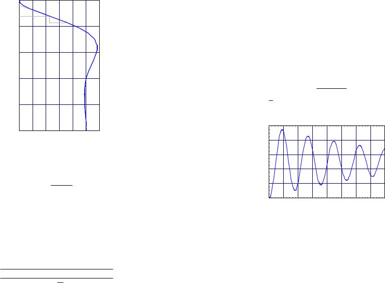
13.1.3 An application of Ziegler-Nicols tuning Let us apply the Ziegler-Nicols tuning methods to an example. Suppose that we have a rotor spinning on a shaft supported by bearings. The angular position of the rotor will satisfy a di erential equation of the form

¨ ˙

Jθ + dθ + kθ = u,

where J is the inertia of the rotor, d accounts for the viscous friction in the bearings, k is the shaft spring constant, and u is the torque applied to the shaft. This then gives a plant transfer function

1

RP (s) = Js2 + ds + k .

Let us take J = 1, d = 101 , and k = 2.

Let us look at the first Ziegler-Nicols method. The step response for the plant is shown in Figure 13.2. One may compute σ and τ graphically. However, in this case it is possible to

	1
	0.8
)	0.6
(t
N,D
1	0.4
	0.2
	2.5	5	7.5	10	12.5	15	17.5	20
				t

Figure 13.2 Step response for rotor on shaft

compute these numerically since the step response is a known function on t. To find tσ one

¨ ≈ determines where 1N,D(tσ) = 0, where (N, D) is the c.f.r. for RP . We compute tσ 1.08 and

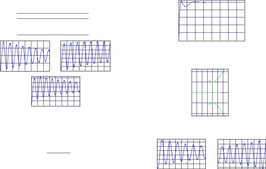
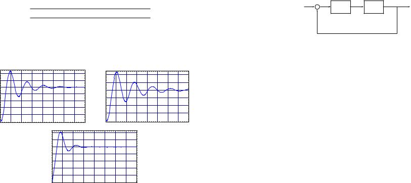
then easily compute σ ≈ 0.70 and τ ≈ 0.40. The values for the P, PI, or PID parameters are shown in Table 13.3. The three corresponding step responses for the closed-loop transfer function, normalised so that they have the same steady state value, are shown in Figure 13.3. Notice that the closed-loop performance is actually rather abysmal. Furthermore, it is quite evident that what is needed in more derivative time. If we arbitrarily set TD = 1 in the PID controller, the resulting step response is shown in Figure 13.4. Note that the response is now more settled. This exercise points out that the Ziegler-Nicols tuning method does not produce guaranteed e ective control laws. Indeed, the system we have utilised is quite benign, and it still needed some adjustment to work well.

22/10/2004 13.1 Ziegler-Nichols tuning for PID controllers 497

Table 13.3 Controller parameters for the rotor example first

Ziegler-Nicols tuning method

		Controller type				Controller parameters
		P				K ≈ 3.83
		PI				K ≈ 3.45, TI ≈ 8.55
		PID				K ≈ 4.60, TI = 0.78, TD ≈ 0.19
									1.4
									1.2
1.5										1
(t)								(t)	0.8
1								Σ
Σ									0.6
1								1
0.5									0.4
									0.2
0										0	2.5	5	7.5	10	12.5	15	17.5	20
2.5	5	7.5	10	12.5	15	17.5	20
			t											t
				1.5
				1.25
			(t)	1
				0.75
			Σ
			1
				0.5
				0.25
				0	2.5	5	7.5	10		12.5	15	17.5	20
								t

Figure 13.3 Normalised step responses for rotor example using first Ziegler-Nicols tuning method: P (top left), PI (top right), and PID (bottom)

Let us now move onto the second of the Ziegler-Nicols methods. We cannot use the rotor example, because it does not satisfy Assumption 13.1. So let us come up with a plant transfer function that does work. An example is

1

RP (s) = s3 + 3s2 + 4s + 1.

In Figure 13.5 is a plot of the behaviour of the poles of the closed-loop system as a function of K with RC(s) = K. As we can see, the roots behave as specified in Assumption 13.1, so we can proceed with that design methodology. The method asks that we find the critical gain Ku for which the roots cross the imaginary axis. One can do this by trial and error, looking at the step response. For example, in Figure 13.6 we plot the step response for two values of K. As we can see, for the plot on the left K < Ku and for the plot on the right K > Ku. One can imagine iteratively finding something quite close to Ku by looking at such plots. However, I found Ku by numerically determining when the real part of the poles for

498

13 Advanced synthesis, including PID synthesis

22/10/2004

	1
	0.8
)	0.6
(t
Σ
1	0.4
	0.2
	0
	2.5	5	7.5	10	12.5	15	17.5	20
				t

Figure 13.4 Normalised step response for rotor example using first

Ziegler-Nicols tuning method and derivative time adjusted to

TD = 1

	2
	1		X
Im	0				X
	-1		X
	-2
	-2.5	-2	-1.5	-1	-0.5	0	0.5
			Re

Figure 13.5 Behaviour of poles for plant RP (s) =	1	and
	s3+3s2+4s+1

RC(s) = K as K varies

										2.5
	1.5
	1.25									2
	1									1.5
(t)									(t)
	0.75									1
Σ									Σ
1									1
	0.5									0.5
	0.25									0
	0									-0.5
	2.5	5	7.5	10	12.5	15	17.5	20		2.5	5	7.5	10	12.5	15	17.5	20
				t									t

Figure 13.6 The step response of the plant RP (s) =	1
	s3+3s2+4s+1

and RC(s) = K for K = 10 (left) and K = 12 (right)

22/10/2004	13.1 Ziegler-Nichols tuning for PID controllers					499
the closed-loop transfer function
		KRP (s)	1
	T (s) =		=
		1 + KRP (s)		s3 + 3s2 + 4s + 1 + K

are zero. The answer is approximately Ku ≈ 11.0. With this value of K the imaginary part

of the poles is then ω ≈ 2.0. Thus we have Tu = 2π ≈ 3.14. The corresponding values for the

ωu

PID parameters are displayed in Table 13.4, and the normalised closed-loop step responses

Table 13.4 Controller parameters for example using second

Ziegler-Nicols tuning method

Controller type Controller parameters

PK ≈ 5.5

PI	K ≈ 4.95, TI ≈ 2.62
PID	K ≈ 6.6, TI = 1.57, TD ≈ 0.39

are shown in Figure 13.7. The PID response is respectable, but might benefit from more

	1.4							1.5
	1.2							1.25
	1							1
(t)
	0.8							(t)
Σ								Σ 0.75
1	0.6							1
	0.4							0.5
	0.2							0.25
	0							0
	2.5	5	7.5	10	12.5	15	17.5	20
				t

2.5	5	7.5	10	12.5	15	17.5	20
			t

	1.4
	1.2
	1
t)	0.8
(
Σ
1	0.6
	0.4
	0.2
	0
	2.5	5	7.5	10	12.5	15	17.5	20
				t

Figure 13.7 Normalised step responses for example using second Ziegler-Nicols tuning method: P (top left), PI (top right), and PID (bottom)

derivative time given its largish overshoot.

500

13 Advanced synthesis, including PID synthesis

22/10/2004

13.2 Synthesis using pole placement

In this section we use a form of pole placement to indicate how to select PID parameters based upon the location of poles. Clearly one cannot choose a PID controller to place the poles anywhere for a general controller. However, in this section we see exactly how well we can do.

13.2.1 Pole placement using polynomials In this section we engage in a rather general discussion of the closed-loop poles using purely polynomial methodology. We consider the standard unity gain feedback loop of Figure 13.8. Our objective is to characterise some

rˆ(s)	RC (s)	RP (s)	yˆ(s)
	−

Figure 13.8 Feedback loop for polynomial pole placement

of the possible closed-loop characteristic polynomials for the system. The main result is the following.

13.2 Theorem Consider the interconnection of Figure 13.8 and let (NP , DP ) be the c.f.r. for RP , supposing deg(DP ) = n. The following statements hold:

(i)if deg(NP ) ≤ n − 1 and if P R[s] is monic and degree 2n − 1, then there exists a proper RC R(s) with c.f.r. (NC, DC) so that the closed-loop characteristic polynomial of the interconnection, DCDP + NP NC, is exactly P ;

(ii)if deg(NP ) ≤ n and if P R[s] is monic and degree 2n, then there exists a strictly proper RC R(s) with c.f.r. (NC, DC) so that the closed-loop characteristic polynomial of the interconnection, DCDP + NP NC, is exactly P .

Proof The following result contains the essential part of the proof.

1 Lemma (Sylvester’s theorem) For polynomials

P (s) = pnsn + pn−1sn−1 + · · · + p1s + p0

Q(s) = qnsn + qn−1sn−1 + · · · + q1s + q0,

with pn2 + qn2 6= 0, define their eliminant as the 2n × 2n matrix

pn

0

· · · 0

qn

0 · · ·

0

pn.−1 p.n

· · · .

q

n.−1 qn · ·.·

0

0

.. .. . . . ..

.. . . . ..

p1

p2

· · ·

pn

q1

q2

· · ·

qn

M(P, Q) =

p1

pn

1

q0

q1

qn

1

.

p0

· · ·

−

· · ·

−

p0

pn

0

q0

qn

0

· · ·

−

2

· · ·

−

2

.. .. . . . ..

.. . . . ..

. .

.

.

.

0

0

p0

0

0

q0

· · ·

· · ·

Then P and Q are coprime if and only if det M(P, Q) 6= 0.

22/10/2004

13.2

Synthesis using pole placement

501

502

13 Advanced synthesis, including PID synthesis

22/10/2004

Proof Note that if P and Q are not coprime then there exists z C so that

Now we proceed with the proof.

P (s) = (s − z)(˜pn−1sn−1 + · · · + p˜1s + p˜0)

(i) Since NP and DP are coprime, their eliminant M(DP , NP ) is invertible by Lemma 1.

Now let P

R[s] be monic and of degree 2n

−

1 and write

n

−

1

+ · · · + q˜1s + q˜0).

Q(s) = (s − z)(˜qn−1s

P (s) = s

2n

−

1

+ p2n−2s

2n

−

2

+

· · · + p1s + p0.

This implies that

Now define a vector in R2n by

(˜qn−1sn−1 + · · · + q˜1s + q˜0)P (s) − (˜pn−1sn−1 + · · · + p˜1s + p˜0)Q(s) = 0.

bn−1

We now balance the coe cients of powers of s in this expression:

.

..

s − : pnq˜n−1

−

qnp˜n−1 = 0

b1

2 .−

2n 2

b0

1 ..

2n

1

p n

1

s

− : pn

−

1q˜n

−

1

+ pnq˜n

−

2

−

qn 1p˜n

−

1

−

qnp˜n

2 = 0

= M(DP , NP )−

p1

.

(13.2)

..

−

−

an

1

.−

p0

.

.

.

s1 : p

q˜ + p

q˜ q

p˜ q

p˜ = 0

0

1

1

0

−

0

1

−

1

0

a1

s

0

: p0q˜0

−

q0q˜0 = 0.

a0

One readily ascertains that this is exactly equivalent to

One verifies by direct computation that the resulting equation

..

..

p n 1

q˜n−1

bn−1

.

.

q˜1

b1

2 .−

q˜

b0

.

0

=

.

M(P, Q)

= 0.

M(DP , NP )

p1

−p˜n

−

1

an−1

.

.

.

.

p0

.

a1

−

p˜1

p˜0

a0

−

This then implies

that

det M(P, Q)

=

0

since

not

all of the coe cients

is exactly the result of equating DCDP + NCNP = P , provided that we define

q˜n−1, . . . , q˜0, p˜n−1, . . . , p˜0 can vanish.

a

n−1

sn−1

+

· · ·

+ a

s + a

Now suppose that det M(P, Q) = 0. This implies that there is a nonzero vector x

R

2n

R

(s) =

1

0

.

C

so that M(P, Q)x = 0. Let us write

sn−1 + bn−2sn−2 + · · · + b1s + b0

q˜n−1

To complete the proof, we must also show that the numerator and denominator in this

finish

expression for RC are coprime.

.

(ii) In this case we take

..

q˜1

P (s) = s2n + p

2n−1

s2n−1 + + p

s + p

,

x =

q˜0

· · ·

1

0

.

−p˜n 1

2n+1

.

.

−

and define a vector in R

by

.

p˜1

bn

−

p˜0

bn 1

−

−

..

p2n−1

n

1

n 1

¯

1 .

Now reversing the argument for the preceding part of the proof shows that

.

= M(DP , NP )−

p2n

.

(13.3)

(˜qn

1s − +

+ q˜1s + q˜0)P (s) = (˜pn

1s −

+

+ p˜1s + p˜0)Q(s)

b0

..

−

· · ·

−

· · ·

Q(s)

q˜n

n

−

1

+

+ q˜1s + q˜0

an

1

p1

1s

.−

=

=

−

n

−

1

+

· · ·

+ p˜1s + p˜0

.

.

p0

P (s) p˜n

−

1s

· · ·

.

a1

a0

Since either P or Q has degree n, it must be the case that P and Q have a common factor. H

22/10/2004	13.2 Synthesis using pole placement					503
¯
Here the matrix M(DP , NP ) is defined by
M¯	(DP , NP ) =	p2n		0t	,	(13.4)
		m(DP )		M(DP , NP )

and where m(DP ) R2n is a vector containing the coe cients of DP , with the coe cient

¯

of sn−1 in the first entry, and with the last n entries being zero. Clearly M(DP , NP ) is invertible since M(DP , NP ) is invertible. Now one checks that if

RC(s) =	an−1sn−1 + · · · + a1s + a0	,
	sn + bn−1sn−1 + · · · + b1s + b0
then this controller satisfies the conclusions of this part of the proposition.

13.3 Remarks 1. This result is analogous to Theorem 10.27 in that it provides an explicit formula, in this case either (13.2) or (13.3), for a stabilising controller for the feedback loop of Figure 13.8. In fact, in each case we can achieve a prescribed characteristic polynomial of a certain type.

2.In Theorem 10.27 the characteristic polynomial had to be of degree 2n and had to be writable as a product of two polynomials (this latter restriction is only a restriction when n is odd). However, in Theorem 13.2 we go this one better because the characteristic polynomial had degree one less, 2n − 1, at least in cases when RP is strictly proper. This means we have a controller whose denominator has one degree less than that of Theorem 10.27. This can be advantageous.

3.One of the things we loose in Theorem 13.2 is the separation principle interpretation

available for Theorem 10.27 (cf. Theorem 10.48).

An example illustrates how to explicitly apply Theorem 13.2.

13.4 Example Let us consider the unstable, nonminimum phase plant

1 − s RP (s) = s2 + 1.

We first wish to design a proper controller that produces the closed-loop characteristic poly-

nomial

P (s) = s3 + 3s2 + 4s + 2.

We determine the eliminant M(DP , NP ) to be
		1		0		0	0
M(DP , NP ) =		0 1 −1 0 .
	0			1		0	1
		1		0		1	−1
An application of (13.2) gives
						4 .
M(DP , NP )−1 3					=
			1			1
		2					2
			4			1
						−

504	13 Advanced synthesis, including PID synthesis																			22/10/2004
This then gives the controller										s − 2
				RC(s) =									.
										s + 4
	T (s) =			RC(s)RP (s)					=			(s − 1)(s − 2)							.
				1 + RC(s)RP (s) s3 + 3s2 + 4s + 2
Note that RC is indeed a proper, but not a strictly proper, controller.
	To achieve a proper controller we use part (ii) of Theorem 13.2. To do this, we must
specify a closed-loop characteristic polynomial of degree 4. Let us go with
			P (s) = s4 + 4s3 + 7s2 + 6s + 2.
				¯	, NP ) in the equation (13.3). Using the description
Next we must determine the matrix M(DP
of this provided in the proof we get
					1			0			0			0		0
		¯			1			1			0			0		0
		M(DP , NP ) =				0 0 1 −1 0 .
					1			1			0			1		−	1
								0			1			0
					0											1
An application of (13.3) gives
							4
				¯										4
								1						1
				M(DP , NP ) 6							=				1 .
								7						5
							2					−3
												−
This then gives the strictly proper controller
				RC(s) =				−s − 3							.
						s2 + 4s + 5
The corresponding closed-loop transfer function is
	T (s) =		RC(s)RP (s)			=						(s + 3)(s − 1)								.
		1 + RC(s)RP (s) s4 + 4s3 + 7s2 + 6s + 2

Note that the order of the two controllers we have designed is as predicted by Theorem 13.2, and are comparable to the order of the plant.

The closed-loop characteristic polynomials are designed to be stable. In Figure 13.9 we show the Nyquist plots for both systems. One can get some idea of the stability margins of the closed-loop system from these.

Let us discuss this a little further by looking into a couple of related results. The first is that if we wish to increase the denominator degree of the controller, we may.

13.5 Corollary Consider the interconnection of Figure 13.8 and let (NP , DP ) be the c.f.r. for RP , supposing deg(DP ) = n ≥ deg(NP ). If P R[s] is monic, of degree k ≥ 2n − 1, and if the coe cient of s2n−1 in P is nonzero, then there exists RC R(s) with c.f.r. (NC, DC) so that the closed-loop characteristic polynomial of the interconnection, DCDP + NP NC, is exactly P .

RP (s) =

22/10/2004		13.2 Synthesis using pole placement		505
	4		4
	3		3
	2		2
	1		1
Im	0	Im	0
	-1		-1
	-2		-2
	-3		-3

-2 -1	0	1	2	3	4	5	-2 -1	0	1	2	3	4	5
		Re							Re

Figure 13.9	Nyquist plots for polynomial pole placement for
RP (s) =	1		for a proper controller (left) and a strictly proper
		s2+1
controller (right)

Proof

Define

DC,1(s) = sk + bk−1sk−1 + · · · + bnsn

by asking that the polynomial D

C,1

D

P2n−

P have degree 2n

−

1. Thus D

C,1

is obtained

k

by equating the coe cients of s

, . . . , s

in the polynomials DC,1DP and P . Now define

˜

1

˜

P =

p2n−1

(P − DC,1DP ). By construction of DC,1, P is monic and has degree 2n − 1. Thus,

by Theorem 13.2, there exists

R˜C(s) =

a˜n−1sn−1 + · · · + a˜1s + a˜0

sn−1 + ˜bn−2sn−2 + · · · + ˜b1s + ˜b0

˜

˜

with the property that DC,2DP + NC,2NP = P , if (NC,2, DC,2) is the c.f.r. for RC. Taking

DC = DC,1 + p2n−1DC,2, NC = p2n−1NC,2, RC =

NC

DC

gives the corollary.

13.6 Remark The controller RC in the corollary will not be unique as it will be, for example, in Theorem 13.2.

Let us now see that the above result works in an example.

13.7 Example (Example 13.4 cont’d) Let us see what happens when we choose a closed-loop characteristic polynomial whose degree is “too high.” Let us suppose that we wish to achieve the closed-loop characteristic polynomial

P (s) = s5 + 5s4 + 12s3 + 16s2 + 12s + 4.

506 13 Advanced synthesis, including PID synthesis 22/10/2004

We should look for a controller of order 5 − 2 = 3. One may verify that the controller

	RC(s) =	−5s3 − 16s2 − 8s − 20
		s3 + 24

achieves the desired characteristic polynomial. However, this is not the only controller that accomplishes this task. Indeed, one may verify that any controller of the form

−5s3 − 16s2 − 8s − 20 + a1(s3 + s2 + s + 1) + a2(s2 + 1)

s3 + 24 + a1(s2 − 1) + a2(s − 1)

will achieve the same characteristic polynomial. Thus we see explicitly how the freedom of the high degree characteristic polynomial plays out in the controller. This may be helpful in practice to fine tune the controller do have certain properties.

It is not surprising that we should be able to achieve a characteristic polynomial of degree higher than that of Theorem 13.2. It is also the case that we can generally expect to do not better. The following result gives this in precise terms.

13.8 Proposition For the interconnection of Figure 13.8, let RP be proper with c.f.r. (NP , DP ) and deg(DP ) = n. If k < 2n − 1 then there exists a monic polynomial P of degree k so that there is no proper controller RC with the property that deg(DC) = k − n, where (NC, DC) is the c.f.r. for RC.

Proof The most general proper controller RC for which deg(DC) = k−n will have 2(n−k+1) undetermined coe cients. The equation DCDP +NCNP = P gives a linear equation in these coe cients by balancing powers of s. This linear equation is one with k + 1 equations in 2(k − n + 1). However, we have

k < 2n − 1 = − k > −2n + 1

= k + 1 > 2k − 2n + 2.

This means that the linear equation for determining the coe cients of RC has more equations than unknowns. Since a linear map from a vector space into one of larger dimension is incapable of being surjective, the proposition follows.

This means that we cannot expect to stabilise a general plant except with a controller whose denominator has comparable degree. This is easily illustrated with an example

13.9 Example (Example 13.4 cont’d) Let us continue with our example where

1 − s s2 + 1.

We wish to show that we cannot find a proper controller RC with the property that the closed-loop characteristic polynomial for the interconnection of Figure 13.8 is an arbitrary Hurwitz polynomial of degree 2. Clearly a proper controller of degree 1 or greater will lead to a closed-loop characteristic polynomial of degree 3 or greater. Thus we may only use a constant controller: RC(s) = K. In this case the closed-loop characteristic polynomial is

readily determined to be

P (s) = s2 − Ks + 1 + K.

22/10/2004	13.2 Synthesis using pole placement	507
1
	X

0.5

Im	0				O
	-0.5
	-1		X
	-1	-0.5	0	0.5	1

Re

Figure 13.10 Locus of roots for s2 −Ks+1+K where K (−1, 0)

Note that this polynomial is Hurwitz only for K (−1, 0). Thus the class of closed-loop characteristic polynomials of degree 2 that we may achieve is limited. Indeed, in Figure 13.10 we show the locus of roots for those values of K for which the closed-loop system is IBIBO stable. The placement of poles is clearly restricted.

13.2.2 Enforcing design considerations Sometimes one wants to design a controller with certain properties. One of the most often encountered of these is that RC have a pole at s = 0 so as to ensure asymptotic tracking of step inputs and rejection of step disturbances. With this in mind, we have the following result.

13.10 Proposition Consider the interconnection of Figure 13.8 and suppose that (NP , DP ) if the c.f.r. for RP . For k N the following statements hold:

(i) if deg(NP ) ≤ n − 1 and if P R[s] is monic and degree 2n + k − 1, then there exists a controller RC R(s) with c.f.r. (NC, DC) with the following properties:

(a)RC is proper;

(b)RC has a pole of order at least k at s = 0;

(c)deg(DC) = n + k − 1;

(d) the closed-loop characteristic polynomial of the interconnection, DCDP + NP NC, is exactly P ;

(ii)if deg(NP ) ≤ n and if P R[s] is monic and degree 2n + k, then there exists a controller RC R(s) with c.f.r. (NC, DC) with the following properties:

(a)RC is strictly proper;

(b)RC has a pole of order at least k at s = 0;

(c)deg(DC) = n + k;

508	13 Advanced synthesis, including PID synthesis		22/10/2004
(d)	the closed-loop characteristic polynomial of the interconnection, DCDP + NP NC,
	is exactly P .
Proof (i) Let us write
	RP (s) =	cn−1sn−1 + · · · + c1s + c0
		sn + dn−1sn−1 + · · · + d1s + d0

and

P (s) = s2n+k−1 + p2n+k−2s2n+k−2 + · · · + p1s + p0.

The idea is the same as in the proof of Theorem 13.2 in that the issue is matching coe cients. The content lies in ascertaining the form of the coe cient matrix. In this case we define a (2n + k) × k matrix Ak(NP ) by

		0			0		· · ·	0	0
	..				..		... ..		..
		.			.			. .
		0			0		· · ·	0	0
Ak(NP ) =	cn		−	1	0		· · ·	0	0
					cn			0	0	.
	cn			2		1
		.−			.−		· · · .		.
	.				.		... .		.
	.				.			.	.
		0			0			c0	c1
		0			0		· · ·	0	c0
							· · ·

The way to assemble Ak(NP ) in practice is to put the components of the polynomial NC into the last column of Ak(NP ), starting with c0 in the last row and working backwards. The next column to the left is made by shifting the last column up one row and placing a zero in the last row. One proceeds in this way until all k columns have been formed. Now define

Mk(DP , NP ) =	0		Ak(NP )	R(2n+k)×(2n+k).
	M(DP	, NP )

One now defines a vector in R2n+k by

	..			p2n+k−1
	bn+k−1
	.

an+.k−1					..
bk		= Mk(DP , NP )−	1		p2n+k−2		.
.					.
					p0
.
a0

	One now checks that if
	RC(s) =	an+k−1sn+k−1 + · · · + a1s + a0	,
		bn+k−1sn+k−1 + · · · + bksk
	then RC has the properties stated in the proposition.
	(ii) Here we write

cnsn + cn−1sn−1 + · · · + c1s + c0 RP (s) = sn + dn−1sn−1 + · · · + d1s + d0

22/10/2004	13.2		Synthesis using pole placement								509	510	13 Advanced synthesis, including PID synthesis							22/10/2004
and	P (s) = s2n+k + p2n+k−1s2n+k−1 +											We then compute
									+ p1s + p0.							1		1
The next step is to define A¯ k(NP )			R(2n+k+1)×k by					· · ·					M1	(DP , NP )		4		9
				0 0				0 0							−1	6	=	1 .
					· · ·												−
				.. .. ..		.	.. ..									2		2
			. .					. .

	0	0 · · · 0 0	Thus we take

¯						cn	0	· · ·		0 0												R (s) = 5s2 − s + 2.
Ak(NP ) =						n.−1	.n			.	.												C	s2 + 9s
					c		c	· · ·		0 0 .
						. .				.	.
						0	0			c0	c1
																		6							6
				. . ...						.	.						The Nyquist plot for the loop gain RCRP is shown in Figure 13.11.
						0	0	· · ·		0	c0
								· · ·
Then we let																		4							4
							A¯ k(NP ) R(2n+k−2)×(2n+k−2),
M¯ k(DP , NP ) =		¯	0															2							2
	M(DP , NP )
¯															2n+k+1	by
where M(DP , NP ) is as defined in (13.4). Then we define a vector in R																	Im	0						Im	0
	..
										p2n+k								-2							-2
	bn+k									p2n+k−1
	.
	bk			¯			, NP )−		1
			= Mk(DP								.			.				-4							-4
an+k		1									..
	. −										p0
.
.
	a0																	-4	-2	0	2		4	6		-4			-2	0	2	4	6
																				Re										Re
The rational function																		20							6
RC(s) = an+k−1sn+k−1 + · · · + a1s + a0
has the desired properties.				bn+ksn+k + · · · + bksk														10							4
Let us apply this in an example, as the proof, as was the proof of Theorem 13.2, is																									2
constructive.																	Im							Im
																		0							0
13.11 Example (Example 13.4 cont’d) We take
			RP (s) = s12 −+s1,															-10							-2
and design a controller with a pole at s = 0 that produces a desired characteristic polynomial.																									-4
First let us achieve a pole of degree k = 1 at the origin. To derive a proper controller, P																		-20
must have degree 2n + k − 1 = 4. Let us take
																		-10		0	10			20		-4			-2	0	2	4	6
	P (s) = s4 + 4s3 + 7s2 + 6s + 2.																			Re										Re
																		Figure 13.11			Nyquist plot for plant RP (s) = 12−s								and controllers
The matrix M1(DP , NP ) is then constructed as in the proof of Proposition 13.10 as																					2					s +1
																			RC(s) =			(top left), RC(s) =				8s2	3s+4			(top right),
						0															5s 2−s+2					3	−2	+19s
							1	−1		0	0								RC(s) =		s +9s					s +5s
																					s3+24s2			(bottom left and right)
						1	0	0		0	0										19s3+8s2+16s+4

M1(DP , NP ) = 1 0 1 −1 0 .

0	1	0	1	−1		If we demand that RC be proper, then we use part (ii) of Proposition 13.10. We must
0	0	0	0	1

22/10/2004	13.2 Synthesis using pole placement															511
now specify a polynomial of degree 2n + k = 5; let us take
P (s) = s5 + 5s4 + 12s3 + 16s2 + 12s + 4.
We compute		0		1	0	0		0				0
		1		0	0	0		0				0
		0		1	0	1		−		1		0
M¯ 1	(DP , NP ) =	1 0 1 −1 0										0			,
		0		0	1	0		1				−	1
				0	0	0		0
		0										1
giving
					5			5
					1			1			.
	M¯ 1(DP , NP )−1 16 =							8
					12			19
				12					3
					4		−
								4
Thus we have
				8s2 − 3s + 4
	RC(s) =								.
			s3 + 5s2 + 19s

One may see the Nyquist plot for the controller in Figure 13.11.

We may also design a controller giving a pole of degree k = 2 at s = 0. This requires the specification of a closed-loop characteristic polynomial of degree 2n + k − 1 = 5; let us take

P (s) = s5 + 5s4 + 12s3 + 16s2 + 12s + 4.

again. We compute
		1	0	0	0		0		0
		0 1 −1			0		0		0
M2	(DP , NP ) =	1 0 1 −1 0							0
		0	1	0	1		1		0
			0	0	0		−
		0					1		1
			0	0	0		0		−
		0							1
and
				1		1
				5	24
				12	=	19
	M2(DP , NP )−1 16					8	.
			12		16
				4		4
Thus we take
		19s3	+ 8s2 + 16s + 4
	RC(s) =							.
			s3 + 24s2

The Nyquist plot for this plant/controller is shown in Figure 13.11. This is not strictly proper, and one may of course apply part (ii) of Proposition 13.10 to get a strictly proper controller. However, it is hopefully clear how to do this at this point.

512

13 Advanced synthesis, including PID synthesis

22/10/2004

13.12 Remark It is interesting to look at the Nyquist plots for the controllers designed in Examples 13.4 and 13.11. First of all, the Nyquist plots get increasingly more complicated as we increase the controller order. One’s ability to design controllers of this complexity with ad hoc methods is quite limited. On the other hand, one can see that the Nyquist plot for the third controller of Example 13.11 (the bottom Nyquist plots in Figure 13.11) has very bad gain and phase margins. One would be suspicious of such a controller, even though the theory tells us that it produces a desirable closed-loop characteristic polynomial. This points out the importance of using all the tools at one’s disposal when designing a controller.

One can also ask that more general polynomials appear in the denominator of RC. Indeed, the proof of Proposition 13.10 can easily, if tediously, be adapted to prove the following result.

13.13 Corollary Consider the interconnection of Figure 13.8 and suppose that (NP , DP ) if the c.f.r. for RP . For F R[s] a monic polynomial of degree k, the following statements hold:

(i) if deg(NP ) ≤ n − 1 and if P R[s] is monic and degree 2n + k − 1, then there exists a controller RC R(s) with c.f.r. (NC, DC) with the following properties:

(a)RC is proper;

(b)DC has F as a factor;

(c)deg(DC) = n + k − 1;

(d) the closed-loop characteristic polynomial of the interconnection, DCDP + NP NC, is exactly P ;

(ii)if deg(NP ) ≤ n and if P R[s] is monic and degree 2n + k, then there exists a controller RC R(s) with c.f.r. (NC, DC) with the following properties:

(a)RC is strictly proper;

(b)DC has F as a factor;

(c)deg(DC) = n + k;

(d) the closed-loop characteristic polynomial of the interconnection, DCDP + NP NC, is exactly P .

Just when one might wish to do this is a matter of circumstance. The following example gives one such instance.

13.14 Example Suppose we are given a plant RP with c.f.r. (NP , DP ) where deg(DP ) = n. A reasonable design specification is that the closed-loop system be able to track well signals of a certain period ω. This would seem to demand that the transfer function from the input to the error should be zero at s = iω. For the interconnection of Figure 13.8 the transfer function from the input to the error is the sensitivity function for the loop,

1

SL(s) = 1 + RC(s)RP (s).

By ensuring that RC has a pole at s = iω, we can ensure that SL(iω) = 0. Thus we should seek a controller of the form

			NC(s)
RC(s) =					.
		2	2	˜
(s			+ ω	)DC(s)

Corollary 13.13 indicates that we can find a proper such controller provided that the closedloop characteristic polynomial is specified to be of degree 2n + k − 1. If the controller is