

Appendix C
Representational Systems for Vector Description
Mathematicians have developed more than a dozen ways of representing the special relationships between physical things. Three of these that are often encountered are through the use of coordinate axes, cylindrical coordinates, and spherical coordinates.
A street map is a two dimensional representation of a town and, like the simple coordinate plane (with an X and a Y axis) that you may have used in school, any location can be represented with a horizontal (X) and vertical (Y) value. A Z-axis can be added to the picture so that any point in space can be identified as P(x,y,z), where the three coordinates are plotted on three axes of the coordinate plane. When you see strange formulae in some antenna book or in some web article discussing electromagnetism (or anything else, for that matter) and you see that 3-dimensional coordinates are presented as an x, y, and z value, you know youʼre using the classic coordinate axes method of representation.
Electronics (and many other disciplines) often involves evaluation of a plane thatʼs wrapped into a circle (a cylinder), like a piece of wire. A second representational system has been developed for
solving equations involving a cylinder. Thereʼs a number and an angle that represents the distance up or down the cylinder at which the point being referenced is located and then the angle based on some 0O on the circle that forms the end of the cylinder. This is called a cylindrical representation (…no surprise there!). When you see an equation where position is represented by two numbers and an angle youʼre working with a cylindrical format, as shown below.
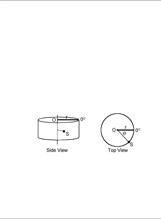
Figure C.1 Vectors Represented Using Cylindrical Coordinates
On the left (Figure C.1 above) is the side view of the representation. A line with length r extends from the vertical line in the middle of the cylinder (at point O) to the circumference of the cylinder. This line has been defined as the 0O line. Below the radial line at O is another line, meeting the circumference of the cylinder at point S. The angle (clearly seen in the top view) between the two lines is shown as θ. A vector represented in cylindrical form would be written S(y,r,θ), giving the point on the vertical y-axis for the origin of the vector, the radius of the cylinder, and the angle formed relative to 0O.
Ultimately, equations often involve points that are naturally in spherical relationships to one-another (like the energy points in a spherically expanding wavefront). The spherical coordinate system (widely used in dealing with electromagnetic radiation equations) is represented below in Figure C.2.
Math and Physics for the 802.11 Wireless LAN Engineer |
92 |
Copyright 2003 - Joseph Bardwell
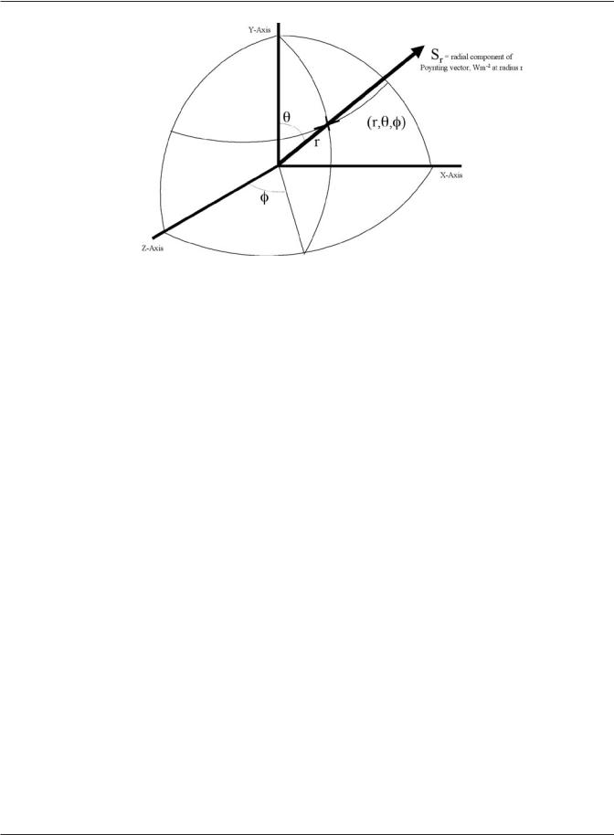
Figure C.2 The Spherical Coordinate System
As you examine the spherical coordinate system figure (above) you see that a particular direction (Sr, the radial component of a Poynting vector in units of Watts per square meter) is shown emanating from the point where the X-, Y-, and Z-axis meet in the center. Instead of representing a point on Sr with an x, y, and z coordinate the angle from the x-axis towards the y-axis is given as θ (theta) and the angle from the x-axis towards the z-axis is given as φ (rho). A point at distance r from the center is represented as (r, θ,φ).
Math and Physics for the 802.11 Wireless LAN Engineer |
93 |
Copyright 2003 - Joseph Bardwell