CHAPTER 3

THE DEVELOPMENT OF THE NUMBER CONCEPT

THE CONCEPT OF NUMBER HAS undergone a long evolution, and today there are several types of “number”. Let us see how this has come about.

The simplest numbers are, of course, the natural or whole numbers 1, 2, 3,...

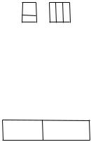
associated with the process of counting. The basic operations of addition and multiplication of natural numbers reflect simple methods of combining assemblages of objects. Thus, for example, in calculating 2 + 3, one starts with 2 = ** objects and juxtapose 3 = *** objects; counting the result yields a set of ** *** = 5 objects. The same number 5 is arrived at by the reverse process of starting with 3 objects and juxtaposing 2 objects: ** *** = *** **. Since this discussion is independent of the particular numbers 2, 3 concerned, we are led to adopt the general rule known as the commutative law of addition: m + n = n + m for any natural numbers m,n. Similar considerations lead to the recognition of the truth of the associative law of addition: (m + n) + p = m + (n + p) for any natural numbers m, n, p. Multiplication now arises from repeated addition: 2 × 3 (also written 2.3), for example, corresponds to the combination of 2 sets of 3 objects. This contains altogether 6 objects, so 2 × 3 = 6. Clearly this combination

***= * * *

**** * *

may also be obtained by combining 3 sets of 2 objects, so 3 × 2 = 6. Thus we are led to adopt the general rule known as the commutative law of multiplication: m × n = n × m for any natural numbers m, n. Similar considerations lead to the recognition of the truth of the associative law of multiplication: m × (n × p) = (m × n) × p for any natural numbers m, n, p. We also recognize an important link between addition and multiplication—the distributive law—which arises in the following way. The expression 2 × (3 + 4), for example, is presented as

*** **** *** ****

We may regard this collection as being composed of two 3s and two 4s, i.e. as

28

THE DEVELOPMENT OF THE NUMBER CONCEPT

29

*******

*******

Thus 2 × (3 + 4) = 2 × 3 + 2 × 4, and we are led to the general assertion m × (n + p) = (m × n) + (m × p) for any natural numbers m, n, p. This is the distributive law for multiplication over addition.

The most important feature of the system of natural numbers is that it satisfies the

Principle of Mathematical Induction, which may be stated as follows. For any property P, if 1 has P and, whenever a natural number n has P, so does n + 1, then every natural number has P. For if the property P satisfies the premise, then 1 has P; from this it follows that 2 has P, from this in turn that 3 has P, and so on for all n. This principle is implicit in Euclid’s proof of the infinitude of the set of prime numbers: for he shows that, if there are n primes, there must be n + 1 primes; and since there is 1 prime, it follows that there are n primes for every n, that is, there are infinitely many primes.

The principle was recognized explicitly by the Italian mathematician Francesco Maurolico (1494 – 1575) in his Arithmetica of 1575. He used it to prove, for example, the fact—known to the Pythagoreans—that

1 + 3 + 5 + … + (2n – 1) = n2.

(1)

This is easily established by mathematical induction. Write P(n) for the property of n asserted by equation (1). Then clearly 1 has P. Now suppose that n has P, i.e., that (1) holds. Then

1 + 3 + 5 + … + (2n – 1) + (2n + 1) = n2 + 2n + 1 = (n + 1)2,

so that n + 1 also has P. From the principle of mathematical induction we conclude that every number has P; in other words, (1) holds for every n.

Chronologically the first enlargement of the system of natural numbers occurred with the adjoining of fractions. These owe their invention to the transition from counting to measuring. Any process of measuring starts with a domain of similar magnitudes, such as, for example, the segments a, b on a straight line. In this case we have, first, a relation a = b of equality or congruence of segments (a and b are said to be congruent if their endpoints can be brought into coincidence) and secondly, an operation + of juxtaposition or addition applicable to any pair a, b of segments producing a segment a + b called their sum. By iterating the operation of addition on a single segment a we obtain for example the segment 4a as the sum a + a + a + a with 4 terms a; in general, for any natural number n, the nth iterate na is defined to be a + a +

... + a with n terms a. In this way each natural number n comes to symbolize an operation, namely, the operation “repeat addition n times.”

The operation of iterated addition on line segments has an inverse called division: given a segment a and a natural number n, there is a unique1 segment x such that nx = a; it is denoted by a/n and is the segment obtained by dividing a into n equal parts.

1By unique here we mean unique up to congruence, that is, all such segments are congruent.

30 CHAPTER 3

Note that, in claiming that division can always be carried out, no matter how large n may be, we are implicitly assuming that our magnitudes—in this case, line segments— are continuous, that is, have no “smallest” parts which are incapable of being further divided.

The operations of iterated addition and division can be combined: thus, for natural numbers m,n and a segment a we define ma/n to be the unique segment x for which ma = nx. The fraction m/n serves then to denote the composite operation “repeat addition m times and divide the result into n equal parts.” Two fractions are accordingly deemed to be equal if the operations they denote are the same, that is, if they both lead to the same

result no matter to what segment a they may be applied: it is then readily	shown that
m/n = p/q if and only if2 mq = np.	(2)

Multiplication of fractions is performed by composition, that is, by carrying out successively the operations denoted by them: thus

(m/n).(p/q) = mp/nq.

(3)

Addition of fractions is not defined quite so readily, but may be performed by noting that, for given m, n, p, q and an arbitrary segment x, we have the identity

mx/n + px/q = [(mq + np)/nq]x,

so that we may define

m/n + p/q = (mq + np)/nq.

(4)

It should be clear that the cogency of this discussion in no way depends upon the specific nature of the magnitudes under consideration; it is only necessary that the operations of (iterated) addition and division be defined on them. Thus we do not need to define special fractions for each domain of magnitudes: just as one system of natural numbers is intended to serve for counting all collections of objects, so, likewise, one system of fractions is intended to serve for measuring all domains of magnitudes. It follows that each pair of natural numbers may be held to determine a unique fraction, and conversely. The definitions of equality, addition and multiplication for fractions conceived as pairs of numbers in this way are then given by (2), (3) and (4) above. It is readily verified that the commutative, associative and distributive laws continue to hold in the system of fractions. Each natural number n may be identified with the fraction n/1, and so regarded as a special kind of fraction (i.e., having unit denominator). Thus the system of fractions becomes an enlargement of the system of natural numbers.

Fractions were invented essentially in order to symbolize the operation inverse to multiplication. Another important development was the introduction of negative numbers, which arise as the result of conceiving of an operation—subtraction—inverse to addition. This is not quite so easily done since, while fractional magnitudes are

2Here we follow the usual convention and omit the dot in multiplication.

THE DEVELOPMENT OF THE NUMBER CONCEPT

31

encountered in everyday life, it is not immediately clear what meaning is to be assigned to the idea of a “negative” magnitude, and as a result negative numbers were not fully accepted until comparatively late in the development of mathematics. Ultimately it came to be seen that negative numbers arise naturally in connection with the measurement of what we may call oriented magnitudes, e.g., financial profits and losses, or directed line segments. We use these latter to illustrate the idea.

Accordingly, we now suppose that each line segment a is assigned a direction or orientation (to the right or left). Equality a = b of directed line segments a,b is then taken to mean that they are not only congruent but also have the same direction. The sum a + b is the directed line segment obtained as follows: if a and b have the same orientation, then a + b is the line segment, with that same orientation, obtained by juxtaposing them. If a and b have opposite orientations, but different lengths, then one, a say, is the greater; we then define a + b to be the line segment with orientation that of a obtained by removing a segment of length b from a. Finally, if a and b have opposite orientations but identical lengths, we define a + b to be a lengthless line segment, that is, a segment 0 whose sum with any line segment a is just a.

Once the sum of directed line segments has been introduced we can define for each natural number n and each a the iterate na as before. This enables us to define the symbol –n by stipulating that –na = (na)*, where, for each segment x, x* denotes the segment obtained by reversing the orientation of x. The symbol –n thus signifies the operation “repeat addition n times and reverse orientation.” Clearly, for any natural number n and any segment a, we have

na + (–na) = 0.

We also introduce the symbol 0 by defining it to symbolize the operation which, upon application to any segment x, reduces it to the lengthless segment 0, i.e.,

0x = 0.

We have thus obtained an enlarged system of symbols ...,–3, –2, 1, 0, 1, 2, 3, ...

each of which denotes a certain operation on directed line segments. Addition and subtraction is defined on these symbols by stipulating that, for each pair p, q, p + q, p – q are to be the unique operations such that, for all x,

(p + q)x = px + qx

(p – q)x = px + (qx)*.

Multiplication is defined, as for fractions, by composing the corresponding operations, i.e. by stipulating that, for any x,

(p.q)x = p(qx).

Clearly the precise nature of the magnitudes we have employed in our discussion is irrelevant, so that—as in the case of fractions—the whole system ...,–3, –2, –1, 0, 1, 2, 3,... may be regarded as autonomous. It is called the set of integers: 1, 2, 3,... are called

32

CHAPTER 3

the positive integers (or natural numbers),...–3, –2, –1 the negative integers and 0 the number zero.

It is easy to verify that the operation of subtraction on integers as defined above is the inverse of addition: i.e., for any integers p, q, p – q is the unique integer x satisfying q + x = p. So the set of integers is, as intended, an enlargement of the set of natural numbers on which the operation of addition has an inverse. It is also readily verified that the commutative, associative, and distributive laws continue to hold in the set of integers.

We have thus shown how to enlarge the set of natural numbers to a system in which multiplication has an inverse—the fractions—and also to one in which addition has an inverse—the integers. If we perform the construction of fractions, only this time starting with the integers instead of the natural numbers (in other words, using directed magnitudes in place of neutral ones), we obtain an enlargement of the system of natural numbers in which both addition and multiplication have inverses (only excepting multiplication by 0). This enlargement is called the system of rational numbers. Any rational number may be represented in the form of a fraction p/n where p is an integer and n is a natural number. The various laws satisfied by the rational numbers may be summarized as follows: for all rational numbers x, y ,z,

x + y = y + x, (x + y) + z = x + (y + z), 0 + x = x + 0 = x, x – x = 0

x.y = y.x, x.(y.z) = (x.y).z, x.1 = 1.x = x, x.(1/x) = 1 (provided x ≠ 0)

x.(y + z) = x.y + x.z.

A system of objects or symbols with two operations + and . defined on it, which contains two distinguished objects 0 and 1, and which satisfies the above conditions is what mathematicians call a field. We may sum up the fundamental character of the system of rational numbers by saying that it constitutes a field. The field of rational numbers is denoted by Q (from German quotient). Note also that the system of positive and negative integers satisfies all the field conditions with the exception of that involving the reciprocal 1/x: such a system is called a ring. The ring of integers is denoted by Z (from German zahl, “number”).

It is helpful to think of the rational numbers as points on a line, in which the positive rationals (i.e. those of the form m/n with m and n positive integers) appear to the right of 0 and the negative rationals (i.e those of the form p/q with p negative and q positive) to the left of 0.

–3 –2 –1 –½ 0 ½ 1 3 2 2 3

This representation displays the ordering of the rational numbers: thus p/m < q/n means that the integer pn is to the left of the integer qm. This ordering turns the rational numbers into what is known as an ordered field.

THE DEVELOPMENT OF THE NUMBER CONCEPT

33

Regarding the rationals as points on a line enables us to divide the line as finely as we please. For example, to represent all rationals of the form m/109 as points on the line, we divide the interval (0, 1) of the line between 0 and 1 into a billion equal pieces; similarly for all other intervals (1, 2), (2, 3),... and the points of subdivision then correspond to fractions of the form m/109. Since the denominator of these fractions can be made arbitrarily large, 1010, 10100, or whatever, thereby producing subdivisions of unlimited fineness, it would be natural to suppose that in this way one would capture as points of subdivision all the points on the line—in other words, that every point is represented by a rational number. Now it is certainly true that rational numbers suffice for all practical purposes of measuring. Moreover, the rational points are dense on the line in the sense that they may be found in any interval (a, b), however small, with rational endpoints a < b. To verify this, observe that the rational number (a + b)/2 lies between a and b. It may actually be inferred from this fact that each such interval contains infinitely many rational points. For if the interval (a, b) contained only finitely many, n say, then we could mark them off as shown, and then any interval between two adjacent points would be free of rational points, contradicting what we have already established.

a

b

All this seems to lend support to the idea that every point on the line is represented by a rational number. The Pythagorean discovery of the incommensurability of the side and diagonal of a square shows, however, that this idea is incorrect. If we take two perpendicular lines OP and PQ of length 1 and use compasses to mark out on the line l a line OR of the same length as OQ then the incommensurability of OP and OQ, and hence also OR, just means that R is not a rational point. In fact, if we designate by r

Q

O

P R

l

the “number” associated with the point R, then we have, by the Pythagorean theorem, r2 = 12 + 12 = 2, so that, replacing r by the customary symbol √2, we conclude that no

rational number is equal to √2, or that √2 is irrational.3

3 The term “irrational” here is to be understood in the sense of “that which cannot be expressed as a ratio” as opposed to its more usual (but related) meaning “contrary to reason”.

34 CHAPTER 3

It can be shown, by arguments similar to that establishing the irrationality of √2, that other numbers formed by root extraction, such as √7, 3 2 (these are solutions to

the equations x2 = 7, x3 = 2) are also irrational. Another number that turns out to be irrational (although this is more difficult to prove) is π, the length of the circumference of a circle of unit diameter.

The fact that not every point on the line corresponds to a rational number means that, if we want to maintain the correspondence between points on a line and “numbers”, the system of rational numbers will have to be enlarged still further. This leads to the system of real numbers. In the last century several methods of constructing this system were devised: here we outline the most straightforward one, which is an extension of the decimal representation of rational numbers. The first thing to observe is that a decimal fraction represents a rational number precisely when it is periodic, i.e., displays a repeating pattern indefinitely after a certain stage (we regard finite decimals as special cases of periodic ones). For example,

6 5 8 = 6.625, 3 7 = 0.428571 428571 .....

The fact is easy to establish: consider the usual long division of N into M which gives the decimal form of M/N. The only possible remainders at each stage of the division are 1, 2,..., N – 1, so that there are just N – 1 possibilities: if any remainder is 0 the process stops and a finite decimal results. It follows that, after at most N divisions, one of the remainders must repeat. Therefore, since each remainder is uniquely determined by its predecessor, the subsequent remainders, and so also the decimal representation itself, must repeat. (Clearly the “repeating block” can have at most N – 1 digits.) Conversely, any periodic decimal represents a rational number. For example, consider

r = 0.90909090...

This may be converted into a fraction by writing

100r = 90.909090... = 90 + r

and subtracting: we obtain 99r = 90, so that r = 90 99 = 1011 . This procedure may be

applied to any periodic decimal: if the repeating block contains m digits we multiply by 10m and subtract just as we have done above.

It follows from this that any nonperiodic decimal must represent an irrational number; it is easy to furnish examples of these, for instance the following decimal containing an increasing number of zeros:

0.101001000100001000001....

Surprisingly, perhaps, no simple rule of this kind exists for constructing the decimal representation of familiar irrational numbers such as √2.

The real numbers are now defined to be the set of all finite or infinite (positive or negative) decimals: considered geometrically the real numbers constitute the geometric

THE DEVELOPMENT OF THE NUMBER CONCEPT

35

continuum or real line. The operations of addition and multiplication can be naturally extended to the real numbers so that, like the rational numbers, they constitute a field,

which we shall denote by the symbol \. So the real numbers resemble the rational

numbers insofar as they are subject to the same operational laws. On the other hand, if we regard the integers as the basic ingredients from which the other numbers are constructed, then our discussion shows that, while each rational number can be defined in terms of just two integers, in general a real number requires infinitely many integers to define it. The fact that infinite processes play an essential role in the construction of the real numbers places them in sharp contrast with the rationals.

In any case the simple definition of real numbers as infinite decimals we have given is not entirely satisfactory since, for one thing, there is no compelling mathematical reason to choose the number 10 as a base for them. We also recall that the real numbers were introduced in order to correspond exactly to points on a line: but how do we know that every such point corresponds to a real number thus defined as a decimal? To establish this it is necessary to show that there are no “gaps” in our set of real numbers, and to define with precision what is to be understood by this assertion. This was carried out in the latter half of the nineteenth century and resulted in the modern theory of real numbers.

The last extension of the concept of number that we shall consider here—the complex numbers—arose, not for geometric reasons, but as the result of attempting to formulate solutions to certain algebraic equations. We have seen that, in order to solve a quadratic equation such as x2 = 2 we need to introduce irrational numbers, and that the rational and irrational numbers together comprise the real numbers. Thinking of the real numbers as points on a line, they are ordered from left to right, with the negative real numbers to the left of zero and the positive ones to the right. Now since the square of any real number, positive or negative, is always positive (or zero) one sees immediately that there can be no real number whose square is negative; in particular, no real number x exists which satisfies x2 = –1. That is, even the simple quadratic equation x2 + 1 = 0 cannot be solved in the system of real numbers. In order to be able to solve such equations we are obliged once again to enlarge our number system. This can be done by formally introducing a new symbol i (called the imaginary4 unit) which is postulated to satisfy the equation

i2 = –1,

that is, i = √–1. We shall suppose that we can form multiples bi of i by any real number b, and sums a + bi for any real number a. A sum of the form a + bi = z is called a complex number: a is called the real part and b the imaginary part, of z. We assume that complex numbers can be added and multiplied in the same way as real numbers, and, in particular, that these operations satisfy the same laws, so that the complex

numbers constitute a field, which we denote by the symbol ^. Calculations with

4 The term “imaginary”—first used in this connection by Descartes—reflects the fact that seventeenthcentury mathematicians considered square roots of negative numbers (such as i = √–1) to be fictitious, the mere product of imagination. In this respect it is to be contrasted with the term “irrational”: q.v. footnote 3.

36

CHAPTER 3

complex numbers can then be performed as with real numbers, replacing i2, wherever it occurs, by –1. Thus, for example, we can compute the product (2 + 3i)(4 + 5i) as follows:

(2 + 3i)(4 + 5i) = 8 + 10i + 12i + 15i2

=(8 - 15) + (10 + 12)i

=–7 + 22i.

Each real number a may be identified with the complex number a + 0i, so that the field of complex numbers may be regarded as an enlargement of the field of real numbers (and thus ultimately as an enlargement of the set of natural numbers).

We observe that two complex numbers z = a + bi and w = c + di are equal if and only if a = c and b = d: this fact is known as the principle of equating real and imaginary parts.

Although the field of complex numbers was introduced just to provide solutions to quadratic equations of the form x2 + a = 0 (which has solutions i√a, –i√a there), much more has actually been gained. In fact, every quadratic equation ax2 + bx + c = 0 (a, b, c real and a ≠ 0) has exactly two complex roots, given by the familiar formula

x = [–b ± √(b2 – 4ac)] /2a.

These roots are real if b2 – 4ac ≥ 0 and complex otherwise. In general, it can be shown

that any algebraic equation—with real or complex coefficients—can be solved in the field of complex numbers. This result, known as the Fundamental Theorem of Algebra, shows that, with the construction of the field of complex numbers, the task of extending the domain of real numbers so as to enable all algebraic equations to be solved has been completed.

Unlike real numbers, complex numbers cannot be represented as points on a line since there is no simple order relation on them. Nevertheless, at the beginning of the nineteenth century they were furnished—independently, and more or less simultaneously, by Caspar Wessel (1745–1818), Jean-Robert Argand (1768–1822) and Karl Friedrich Gauss (1777–1855)—with a simple geometric interpretation as points in a plane. In this interpretation, the complex number a + bi is represented as the point z in the plane with rectangular coordinates (a ,b). In this way any complex number is

a + bi = z

b

a

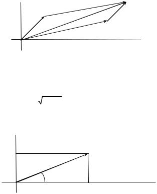
uniquely correlated with a point in what is known as the complex plane (or Argand diagram). Addition and multiplication of complex numbers then admit simple geometric interpretations. In the case of addition, we regard a + bi as a displacement (or vector) from the origin (0, 0) to (a, b). Thus the sum

THE DEVELOPMENT OF THE NUMBER CONCEPT

37

(a + bi) + (c + di) = (a + c) + (b + d)i

is the point in the complex plane obtained by the vector (parallelogram) addition law:

(a + bi) + (c + di)

c + di

a + bi

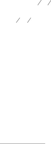
To explain the geometric interpretation of multiplication of complex numbers we shall need to introduce their trigonometric representation. Referring to the figure immediately below, if we denote the distance of the point z from the origin O by r, then

by the Pythagorean theorem r = a2 +b2 . This real number is called the modulus of z, and is written |z|. Note that the distance between the points represented by the complex

a + bi = z

br

θ

O

a

numbers z and z′is then |z –z′|. The angle θ that the line Oz makes with the positive x-

axis is called the argument or amplitude of z. In trigonometry the sine and cosine of the angle θ are defined by

sin θ = b/r cos θ = a/r,

so that a = r cos θ, b = r sin θ. (Note that then sin2 θ + cos2 θ = (a2 + b2)/r2 = 1.) This yields the trigonometrical form of z, namely

z = a + bi = r(cos θ + i sin θ).

(5)

Thus, for example, if z = 1 + i, then r = √2, θ = 45°, so that

38

CHAPTER 3

1 + i = √2(cos 45° + i sin 45°).

The representation (5) yields a simple expression for the reciprocal of a complex number. In fact, if z is given as in (5), we find that, assuming r ≠ 0,

					1	z	= 1	r	.(cos θ – i sin θ).
This follows from the calculation
z.	1	z	= r. 1	r	(cos θ + i sin θ)(cos θ – i sin θ) = cos2 θ + sin2 θ = 1.

Now suppose that we wish to multiply the complex numbers z = r(cos θ + i sin θ)

and z′= r′(cos θ′+ i sin θ′). Then
zz′= rr′[(cos θ cos θ′ sin θ sin θ′) + i(cos θ sin θ′+ sin θ cos θ′)].
Since the sine and cosine functions satisfy the fundamental addition relations
cos(θ + θ′) = cos θ cos θ′ – sin θ sin θ′
sin(θ + θ′) = cos θ sin θ′ + sin θ cos θ′,
we infer that
zz′ = rr′[cos(θ + θ′) + i sin(θ + θ′)].	(6)

But this is the trigonometrical form of the complex number with modulus rr′ and argument θ + θ′. Accordingly, to multiply complex numbers one multiplies their

moduli and adds their angles5. Multiplication by a complex number of modulus 1 and argument θ thus corresponds precisely to rotation through the angle θ. In particular, multiplication by i = cos 90° + i sin 90° corresponds to rotation through a right angle.

Taking z = z′ in (6), we get

z2 = r2(cos 2θ + i sin 2θ),

and, multiplying this result again by z,

z3 = r3(cos 3θ + i sin 3θ).

5 So the product of complex numbers is a “complex” of multiplication and addition.

THE DEVELOPMENT OF THE NUMBER CONCEPT

39

Continuing indefinitely in this way, we obtain, for arbitrary n,

zn = rn(cos nθ + i sin nθ).

Putting r = 1, we obtain the memorable formula of A. De Moivre (1667–1754)

(cos θ + i sin θ)n = cos nθ + i sin nθ.

Using De Moivre’s formula we can determine the roots of the equation xn – 1 = 0—the nth roots of unity—in the field of complex numbers. Taking θ = m.360°/n for m = 1, 2, …, n, we see that nθ is a multiple of 360°, so that cos nθ = 1, sin nθ = 0. The formula then gives

(cos θ + i sin θ)n = cos nθ + i sin nθ = 1 + 0i = 1.

Accordingly the roots of the equation xn – 1 = 0 are

x = cos(m.360°/n) + i sin(m.360°/n)

for m = 1, 2, 3, …, n. Writing α for the root cos(360°/n) + i sin(360°/n), we see that the

roots may be represented as 1, α2, …, αn–1 (in general, this is true for any root α ≠ 1.) Geometrically the values of x are represented by the vertices of the regular n–sided polygon inscribed in the unit circle, and so the equation xn – 1 = 0 is known as the cyclotomic—“circle cutting”—equation.

THE THEORY OF NUMBERS

Number theory, hailed by Gauss as the Queen of Mathematics, abounds in problems that are easy to state, but extremely difficult to solve, and which have been the source of some of the deepest mathematical investigations. We outline a few of these problems, all of which have intrigued mathematicians for centuries.

Perfect Numbers

We recall that a number6 is perfect if it is the sum of its proper divisors. The first four perfect numbers, viz., 6, 28, 496, 8128 were known to the Greeks, and the next, 33550336, appears in a medieval manuscript. In Book IX of Euclid’s Elements it is proved (expressed in modern symbolism) that if 2k – 1 is prime, then 2k–1(2k – 1) is perfect. In the eighteenth century Euler proved what amounts to a converse for even

6Throughout our discussion of number theory, the term “number” or “integer” will always mean “natural number”.

40

CHAPTER 3

perfect numbers, namely, that any such number is of the form 2p–1(2p – 1), where both p and 2p – 1 are prime. Prime numbers of the form 2p – 1 are called Mersenne primes after Marin Mersenne (1588–1648). The complete list of currently known prime numbers p such that 2p – 1 is (a Mersenne) prime is: 2, 3, 5, 7, 3, 17, 19, 31, 61, 89, 107, 127, 521, 607, 1279, 2203, 2281, 3217, 4253, 4423, 9689, 9941, 11213, 19937, 21701, 23209, 44497, 86243, 32049, 216091, 756839, 859433, 1257787, 1398269; to each of these there corresponds a perfect number. Thus the largest perfect number known (as of 1997) is

21398268(21398269 – 1).

One may naturally ask: do the perfect numbers go on forever? Or is there a largest one? The answer to this question is still unknown. Another question which remains unanswered is: do odd perfect numbers exist? One of the few facts that has been established about these elusive numbers is that none smaller than 10200 can exist.

Prime Numbers

Prime numbers play the same role with respect to multiplication as does the number 1 with respect to addition: just as every number is uniquely expressible as a sum of 1s, so every number is uniquely expressible as a product of primes. (Of course, the first fact is trivial, but the second—the fundamental theorem of arithmetic—is not.) We have already pointed out that the Greeks knew that the sequence of primes

2, 3, 5, 7, 11, 13, 17, 19, 23, ...

is unending. As we recall, this is proved by showing that, for any number n, there is a prime between n and n! + 1 (where n! = 1 × 2 × 3 × ...× n). In 1850 the result was greatly improved by the Russian mathematician P. Chebychev (1821–1894) who

showed that, for any number n ≥ 2, there is always a prime between n and 2n. This is

the case despite the fact that, as we proceed through the number sequence, the primes become very sparsely distributed indeed. This becomes apparent when it is observed that, for any number n, we can find a sequence of n consecutive numbers none of which is prime. (Consider, for example, the sequence (n+2)!+2, (n+2)!+3,..., (n+2)!+(n+1).)

Two famous results concerning prime numbers are Fermat’s and Wilson’s Theorems. These are most conveniently stated in terms of the idea of congruence of numbers. If m is a positive integer, and a,b integers (positive, negative, or zero), we say that a is congruent to b modulo m and write

a ≡ b (mod m)

if m divides a – b. It is readily shown that a ≡ b (mod m) precisely when a and b leave the same remainder on division by m. Fermat’s Theorem, stated in 1640 by Pierre de Fermat (1601–1665) is the assertion that, if p is prime, then for any number a,

THE DEVELOPMENT OF THE NUMBER CONCEPT

41

ap ≡ a (mod p).

Wilson’s Theorem (actually proved by Lagrange) is the assertion that, for any number n, n is prime if and only if (n – 1)! ≡ –1 (mod n). 7

Many attempts have been made to find simple arithmetical formulas which yield only primes. For example, in the seventeenth century Fermat advanced the famous conjecture that all numbers of the form

F(n) = 22n +1

are prime. Indeed, for n = 1, 2, 3, 4 we have F(1) = 5, F(2) = 17, F(3) = 257, F(4) = 65537, all of which are prime. However, in 1732 Euler discovered the factorization F(5) = 641 × 6700417, so that F(5) is not a prime. And it is now known that all F(n)

with 5 ≤ n ≤ 19 are composite (i.e., are not prime). So it is possible, although not so far established, that F(n) is composite for all n ≥ 5, and Fermat (almost) totally wrong.

Euler discovered the remarkable polynomial n2 – n + 41, which yields primes for n = 1, 2,..., 40. The polynomial n2 –79n + 1601 yields primes for all values of n below 80. In the nineteen seventies explicit polynomials (in several variables) were constructed whose values comprise all the prime numbers. Thus, even though these polynomials are too complex to be of any practical use, in a formal sense the dream of number theorists of producing an algebraic formula yielding all the primes has finally been realized.

A decisive step was taken in the investigation of prime numbers when attention shifted from the problem of finding exact mathematical formulas yielding all the primes to the question of how the primes are, on the average, dispersed through the integers. While the primes are individually distributed with extreme irregularity, a remarkable regularity emerges when one considers the likelihood of a given number being prime. Writing π(n) for the number of primes among the integers 1, 2, ..., n, then the likelihood or probability8 that a number selected at random from the first n integers will be prime may be identified with the quotient π(n)/n. The prime number theorem which expresses the regular behaviour of this quotient is regarded as one of the greatest discoveries in mathematics. In order to state it we need to define the concept of natural logarithm of a number. To do this we take two perpendicular axes in a plane and consider the curve comprising all points in the plane the product of whose distances x and y from these axes is equal to 1. In terms of the coordinates (x ,y) of the point, this curve—a rectangular hyperbola—has equation xy = 1 and looks like this:

7 Proving this theorem in one direction is easy, for if n has a factor d with 1 < d < n, then d cannot divide (n – 1)! + 1, and so neither can n.

8If a given event can occur in m ways and fail to occur in n ways, and if each of the m + n ways is equally likely, the probability of the event occurring is defined to be m/(m + n).

42

CHAPTER 3

log(n)

1

n

We now define log(n), the natural logarithm of n, to be the area in this figure bounded by the hyperbola, the x-axis, and the vertical lines x = 1 and x = n. In the late eighteenth century, through studying tables of prime numbers, Gauss observed that the quotient π(n)/n is roughly equal to 1/log(n), and that the approximation appears to improve with increasing n. Such empirical evidence led him to conjecture that π(n)/n is “asymptotically equal” to 1/log(n). By this we mean that the ratio of these two quantities, that is,

	π(n) n	=	π(n)
	1 log(n)		n log(n)

can be made to come as close to 1 as we please by making n sufficiently large. Although easily understood, proving Gauss' conjecture turned out to be extremely difficult, and indeed a rigorous proof was not forthcoming until 1896, nearly a century later.

Thus the problem of the average distribution of prime numbers has achieved a satisfactory solution. There remain, however, many other conjectures concerning prime numbers whose truth is suggested by empirical evidence but which have so far resisted final proof (or refutation).

One of these is the celebrated Goldbach conjecture. In a letter to Euler written in 1742 the amateur mathematician C. Goldbach (1690–1764) observed that every even number (except 2) that he had tested could be expressed as the sum of two primes: for example, 4 = 2 + 2, 12 = 5 + 7, 48 = 29 + 19, etc. Goldbach asked Euler whether he could prove this to be true for all even numbers, or if he could provide an example to refute it. Euler never came up with an answer, and the problem—Goldbach’s conjecture—still awaits solution. The empirical evidence for the truth of this conjecture is very strong, but the fact that it involves the addition of primes, while these themselves are defined in terms of multiplication, makes the construction of a rigorous proof no easy matter. In fact, it is rarely simple to establish connections between the multiplicative and additive properties of the integers. Nevertheless, some progress with Goldbach's problem has been made: we now know, for example, that every sufficiently

THE DEVELOPMENT OF THE NUMBER CONCEPT

43

large9 even number may be expressed as the sum of no more than four primes, and also as the sum of a prime and a number with no more than two prime factors.

A final “prime riddle” on which little or no progress has been made is the twin prime conjecture, that is, the assertion that there are arbitrarily large prime numbers p for which p + 2 is also prime. This problem differs in logical status from Goldbach's conjecture in that it cannot be refuted by supplying a single counterexample.

Sums of Powers

In 1770 the English algebraist Edward Waring (1734–1798) advanced the claim that every number was the sum of four squares, nine cubes, 19 fourth powers, etc. This was pure conjecture on his part, but not long afterwards Lagrange succeeded in establishing the correctness of Waring's claim for squares (a claim which had actually been made much earlier by Fermat). It was not until 1909, however, that Waring’s assertion was shown (by Hilbert) to be true in the general sense that, for any number k, there exists a number s such that every integer can be expressed as a sum of no more than s kth powers. The problem of determining the least such number w(k) for arbitrary k is known as Waring’s problem. It is now known how to calculate w(k) for all k, with the

exception, curiously, of k = 4, although it is known that w(4) ≤ 19 (so that Waring was right in this case). For all k such that 1 ≤ k ≤ 200000, except k = 4, it turns out that

w(k) = 2k – 2 + the largest integer < (3 2)k .

Now although w(3) = 9, very few integers actually require as many as 9 cubes to represent them: in fact, only 23 and 239 require so many. The largest integer requiring eight cubes is 454, and inspection reveals that the proportion of integers requiring seven cubes decreases as we proceed through them. Numbers like 23, 239, 454 thus seem to be no more than irritating anomalies. In view of this it is more interesting to consider, instead of w(k), the number W(k) defined to be the least value of s for which every sufficiently large integer can be written as a sum of no more than s kth powers. It is known that W(2) = 4, and, strangely, the only other value of k for which W(k) is known with certainty is k = 4, the one value of k for which w(k) is unknown. In fact W(4) = 16; all that is known about W(k) for other values of k is that they cannot exceed

a certain size: for example, W(3) ≤ 7 and W(5) ≤ 23. The most that is known in general about W(k) is that

k + 1 ≤ W(k) ≤ k(3log(k) + 11),

9By a “sufficiently large” number of a given type we mean a number of that type exceeding some fixed number specified in advance.

44

CHAPTER 3

the right hand inequality being extremely difficult to prove. Waring’s problem is still an active issue in number theory.

Fermat’s Last Theorem

It was Fermat's habit to record his observations in the margins of his copies of mathematical works. In commenting on a problem in Diophantus’s Arithmetic, asking for the solution in rational numbers of the equation x2 + y2 = a2, Fermat remarked that he had found a “truly marvellous demonstration” of the assertion that, by contrast, there

are no integral solutions to any of the equations xn + yn = zn for n ≥ 3, adding that,

unfortunately, the margin was “too narrow to contain” the demonstration. This assertion is often called Fermat’s Last Theorem, but it would be more apt to term it “Fermat’s conjecture”, since it is not known whether he actually had a correct proof of it. It seems unlikely that he did since the best efforts of his successors to prove it failed until very recently. Fermat himself gave an explicit proof for the case n = 4, and Euler proved the case n = 3 between 1753 and 1770 (a lacuna in the proof later being filled by Legendre). Around 1825 proofs for n = 5 were independently formulated by Legendre and Dirichlet, and in 1839 Lamé proved the theorem for n = 7. In the nineteenth century significant advances in the study of the problem were made by the German mathematician E. Kummer, which led to the development of the theory of algebraic numbers (q.v. Chapter 6). Before the First World War, a substantial prize (the value of which was subsequently wiped out by inflation) was offered in Germany for a complete proof, and many amateurs contributed attempted solutions. Legend has it that the number theorist Edmund Landau (1877–1938) had postcards printed which read: “Dear Sir or Madam: Your attempted proof of Fermat’s Theorem has been received and is hereby returned. The first mistake occurs on page ___, line ___.” These he would give to his students to fill in the missing numbers. In 1994, the efforts of mathematicians of the last three centuries to prove Fermat’s Theorem culminated in Andrew Wiles' successful complete proof. This is of great depth and complexity, drawing on results and techniques from several areas of mathematics ouside number theory which had not been developed in Fermat’s day. Nevertheless, we cannot be entirely certain that Fermat—a great mathematician—did not possess a proof himself, one which his successors have so far failed to see.

The number π

The real number π is defined10 to be the length of the circumference of a circle of unit diameter, and is thus the ratio of the length of the circumference of any circle to its

10The general use of the symbol π in its familiar mathematical sense was first adopted by Euler in 1737.

THE DEVELOPMENT OF THE NUMBER CONCEPT

45

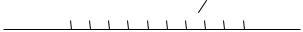
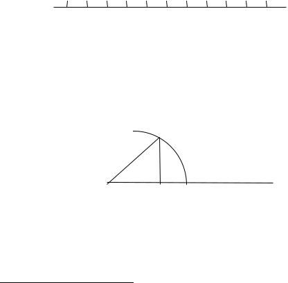
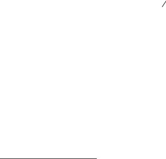
diameter. It may also be defined as the area of a circle of unit radius, since, as was known to the Greeks, the area of a circle is equal to one half of the product of its radius by its circumference. It is of interest to see how it is believed this result was first discovered. If a circle of radius r and circumference c is divided into a large number of segments, as in the figure below, then, if there are sufficiently many of them, each may be taken as an actual triangle. In other words, we may take the circle to be a regular polygon with a large number of sides. This polygon can now be opened out to give

a serrated figure in which the height of each serration is r and the length of the base is c. But clearly the area of this figure, and hence also of the original circle, is one half of

the area of the rectangle with the same base and height, i.e. ½rc.

The problem of computing π has a very long history. In ancient Egypt its value was often taken as 3, but the better value (4 3)4 = 3.1604... appears in the Rhind Papyrus.

The first truly scientific attempt to compute π seems, however, to have been made by Archimedes around 240 B.C. In his work The Measurement of a Circle, (mentioned in the previous chapter) by evaluating the perimeters of regular inscribed and circumscribed polygons he shows that π falls between 223 71 and 227 , so that, to two

decimal places, π = 3.14. The first value of π better than that of Archimedes was obtained by Ptolemy (c.85–165) around 150 A.D. in his great astronomical work popularly known through its Arabic name The Almagest. Ptolemy obtained the value 377/120 = 3.1416. Around 480 A.D. the Chinese mathematician Tsu Ch'ung-chih (430501) obtained the unusual rational approximation 355113 = 3.1415929, correct to six

decimal places, and in 530 the Hindu mathematician Aryabhata (c.475–550) gave the fraction 6283220000 = 3.1416 as an approximate value for π. In 1150 the Hindu mathematician Bhaskara (1114–1185) produced several approximations for π: 39271250 as an accurate value, and √10 for ordinary calculations, inter alia.

In 1579 François Viète (1540-1603) determined π correct to nine decimal places by applying Archimedes’ method to polygons having 6.216 = 393296 sides. Also due to him is the curious “infinite product” in which, by taking the product of sufficiently many terms on the right, we may approximate to π as closely as we please:

2	2		2	.	2
2			2 + 2		2 + 2 +	2

46

CHAPTER 3

In 1650 John Wallis (1616–1703) also obtained π in the form of an infinite product

12 π =	2 2 4 4 6 6 8	,
	1 3 3 5 5 7 7

which was converted by Lord Brouncker (c.1620–1684) into the “continued fraction”

4	π	=1 +			12
				+	3		2
		2
					2 +			52
								+ ...
					2

In 1671 James Gregory (1638–1675) obtained π as an “infinite series” (see Chapter 9)

14 π =1 − 13 + 15 − 17 + ...

in which, by adding and subtracting sufficiently many terms on the right, we can approximate to 14 π as closely as we please (albeit very slowly).

Other remarkable series involving π are those obtained in the eighteenth century by Euler:

16 π2 =1 + 122 + 132 + 142 + ...

and

18 π2 =1 + 132 + 152 + 172 + ...

A major step in the elucidation of the nature of π was taken in 1767 by Johann Heinrich Lambert (1728–1777) when he established its irrationality. In 1794 AdrienMarie Legendre (1752–1833) took this further by showing that π2 is irrational, so that π cannot be the square root of a rational number.

An intriguing connection between π and the concept of probability was noted in 1777 by the Comte de Buffon (1707–1788) through the devising of his famous needle experiment. Buffon showed that, if a needle is dropped at random on a uniform parallel ruled surface on which the distance between successive lines coincides with the length of the needle, then the probability of the needle falling across one of the lines is 2/π. The incongruous presence of π here results from the fact that the outcomes of the experiment depend not only on the fallen needle’s position, but also on the angle it makes with the lines on the surface, and angles are measured by lengths of circular arcs, i.e. in terms of π. By noting the number of successful outcomes of a large number of trials of the experiment, one obtains a value for the probability and hence also an

THE DEVELOPMENT OF THE NUMBER CONCEPT

47

approximate value for π . In 1901 the experiment performed with 3400 tosses of the needle led to an amazingly accurate estimate of π correct to six decimal places!

In 1882 C. L. F. Lindemann (1852–1939) proved the decisive result that π is transcendental, that is, not a root of any polynomial with integer coefficients. This showed conclusively that the ancient problem of squaring the circle cannot be solved with Euclidean tools.

WHAT ARE NUMBERS?

While there is universal agreement on the rules for calculating with the natural numbers, there has been a surprising lack of unanimity concerning what they actually are. To Aristotle, for example, a number was an arithmos, a plurality of definite things, a collection of indivisible “units.” The Greeks did not regard 1 (let alone 0) as a “number” since it is a unit rather than a plurality. Neither could they conceive of fractions as numbers since the unit is indivisible: numbers for them were discrete entities to be distinguished absolutely from geometric magnitudes which are continuous and can be divided indefinitely. Although Diophantus in the third century B.C. had suggested that the unit be treated as divisible to facilitate the solution of certain problems, it was not until the sixteenth century that the Greek concept of number as an assemblage of discrete units began seriously to give way to the idea of number as a symbol indicating quantity in general, including continuous quantity. Thus Simon Stevin (1548–1620) avers that number is not to be identified with discontinuous quantity, and that to a continuous magnitude there corresponds a continuous number. Stevin regards not only 0 and 1, but fractions and even irrational numbers such as √2 as “numbers.” His successors were to take up this idea with gusto.

Although this enlargement of the concept of number proved a valuable stimulus for the development of mathematics, it had at the same time the paradoxical effect of rendering obscure the nature of the original “numbers”—the natural numbers—that had given birth to the new concepts. For while fractions, negative numbers and the like are essentially symbols signalizing the effect of operations11, the natural numbers seem to have a more immediate, concrete, even eidetic character—as the Greeks acknowledged in their identification of numbers with arithmoi.

In the last quarter of the nineteenth century these issues excited a new interest among mathematicians, leading to the publication of several works in which attempts were made to clarify the nature of number, and to put the whole subject of arithmetic on a logical basis. The first of these to appear was Gottlob Frege’s (1848 – 1925) The Foundations of Arithmetic, which was published in 1884. This book has been called the first philosophically sound discussion of the concept of number in Western civilization, an assessment with which it would be hard to disagree. In it Frege subjects the views on the nature of number of his predecessors and contemporaries to merciless analysis,

11 It was the fact that imaginary and complex numbers could not (at first) be conceived of as operations that prevented them from being regarded as “numbers” —even in this extended sense—until the end of the eighteenth century.

48

CHAPTER 3

finally rejecting them all, and proposes in their place his own compellingly subtle theory. It is worth quoting his summary of the difficulties standing in the way of arriving at a satisfactory account of number.

Number is not abstracted from things in the way that colour, weight and hardness are, nor is it a property of things in the sense that they are. But when we make an assertion of number, what is that of which we assert something? This question remained unanswered.

Number is not anything physical, but nor is it anything subjective (an idea).

Number does not result from the annexing of thing to thing. It makes no difference even if we assign a fresh name to each act of annexation.

The terms “multitude”, “set” and “plurality” are unsuitable, owing to their vagueness, for use in defining number.

In considering the terms one and unit, we left unanswered the question: How are we to curb the arbitrariness of our ways of regarding things, which threatens to obliterate every distinction between one and many?

Being isolated, being undivided, being incapable of dissection—none of these can serve as a criterion for what we express by the word “one”.

If we call the things to be counted units, then the assertion that units are identical is, if made without qualification, false. That they are identical in this respect or that is true enough but of no interest. It is actually necessary that the things to be counted should be different if number is to get beyond 1.

We [are] thus forced, it seem[s], to ascribe to units two contradictory qualities, namely identity and distinguishability.

A distinction must be made between one and unit. The word “one”, as the proper name of an object of mathematical study, does not admit of a plural. Consequently, it is nonsense to make numbers result from the putting together of ones. The plus symbol in 1 + 1 = 2 cannot mean such a putting together.

The account of number Frege puts forward in The Foundations of Arithmetic has several key features. First, by “number” he means cardinal number, that is numbers such as one, two, three which answer to the question “how many?”, as opposed to ordinal number such as first, second, third which answer to the question “what position in a series?”. Secondly, and relatedly, numbers are to be treated as definite objects, rather than predicates or properties. Finally, and crucially, numbers are to be conceived as attaching not directly to things, but rather to concepts. Thus, for example, in saying that there are five fingers on my right hand I am assigning the number five to the concept “finger on my right hand”, rather than to the actual assemblage of fingers itself. Frege thus maintains that numbers only become assigned to things in an indirect way: first the concept of the thing is abstracted from the given things, and then the number is assigned to the concept. Frege suggests that the concept itself is the “unit” in respect of the number assigned to it. Thus, for example, in saying that there are five fingers on my right hand the relevant unit is the concept “finger”, but in asserting that there are fourteen joints on the same hand the unit is the concept “joint”. This, he claims, makes it easy to reconcile the identity of units with their distinguishability, for here the word “unit” is being used in a double sense. First, it is used in the sense of “concept”, and since one single concept, for example “finger”, attaches to the collection to which the number is being assigned, the “units” in this sense are identical. On the other hand, when we assert that units are distinguishable, we mean “unit” in the sense of “thing numbered”, and these are, for the purpose of numeration, always taken as distinct.

THE DEVELOPMENT OF THE NUMBER CONCEPT

49

Thus Frege has explicated how numbers come to be assigned, but he has not yet determined what they actually are. To do this he employs the familiar fact that two collections of things have the same number precisely when the members of one collection can be paired off with those of the other in such a way that both are exhausted: in this event we say that the two collections are equinumerous. This term may be extended to concepts by saying that two concepts are equinumerous if the collections of objects to which the concepts respectively attach are equinumerous. Thus, for example, the concepts “side of a triangle” and “vertices of a triangle” are equinumerous in this sense. Frege then defines the number assigned to a given concept to be the collection of all concepts equinumerous with the given one12. Thus for Frege a number corresponds to a collection of concepts. The specific natural numbers 0, 1, 2,… can then be defined as follows:

0 is the number assigned to the concept “not identical with itself”13; 1 is the number assigned to the concept “identical with 0”;

2 is the number assigned to the concept “identical with 0 or identical with 1” ….

n is the number assigned to the concept “identical with 0 or identical with 1 or identical with 2 or … or identical with n – 1”.

Frege admits that it may seem somewhat strange to define a number as a collection of concepts, but he goes on to show that from his definition all the usual facts about numbers (including the Principle of Mathematical Induction) can be derived. It was highly unfortunate that one of the logical assumptions on which Frege’s account of number rested turned out to be inconsistent; however, later investigations have shown that his framework can be salvaged: see Chapter 12.

In 1888 a second major work on the foundations of arithmetic was published—The Nature and Meaning of Numbers by the German mathematician Richard Dedekind

(1831–1916). Unlike Frege, Dedekind is not concerned to give a completely explicit definition of natural number itself; instead, he specifies a structure (based on the primitive notion of set or class) which possesses the essential properties of the whole sequence of natural numbers, and then obtains the natural numbers themselves by an act of mental abstraction.

To grasp the underlying motivation of Dedekind’s approach, consider the set ` of natural numbers {1, 2, 3,…},where, following Dedekind, we take the sequence as beginning with 1. With each number n we associate its successor n′= n + 1. Dedekind generalizes this in the following way. Instead of ` he takes an arbitrary set S (which he

calls a “system”) and instead of the successor operation an arbitrary one-one function ϕ from S into itself (for definitions of these terms, see Chapter 4). Now, for an arbitrary

element s of S, write s′ for ϕ(s) and if A is any subset of S, write A′ for the set

12 Strictly speaking, Frege defines this number to be what is known as the extension of the concept “equinumerous to the given concept”: see Chapter 12 for further details.

13 It will be seen that the concept “not identical with itself” attaches to no object, so that the corresponding number is indeed zero.

50

CHAPTER 3

consisting of all elements of the form s′ for s in A. Clearly `′ is included in `. Dedekind accordingly defines a chain to be a subset K of S such that K′ is included in K. Since, intuitively, ` is the smallest chain which contains the number 1, he defines

by analogy the chain of a subset A of S, written A0 , to be the smallest chain which includes A, that is, the common part of all chains which include A. Dedekind next introduces the concept of simply infinite system: by this he means a set S together with an operation ϕ of S into itself and an element 1 of S such that: (i) S = 10, (ii) the

element 1 is not contained in S′, (iii) the operation ϕ is one-one. Finally he makes the

Definition. If in the consideration of a simply infinite system ` set in order by a

transformation ϕ we entirely neglect the special character of the elements; simply retaining their distinguishability and taking into account only the relation to one another in which they are placed by the order-setting transformation ϕ, then are these elements called natural numbers or ordinal numbers or simply numbers, and the base element 1 is called the basenumber of the number-series N. With reference to this freeing the elements from every other content (abstraction) we are justified in calling numbers a free creation of the human mind. The relations or laws which are derived entirely from the conditions [(i), (ii), (iii) above] and therefore are always the same in all ordered simply infinite systems, whatever names may happen to be given to the individual elements … form the first object of the science of numbers or arithmetic.

The Principle of Mathematical Induction is now an immediate consequence of this definition of natural numbers. For if P is any property defined on the members of a

simply infinite system ` such that 1 has P, and, whenever a has P, so does a′, then clearly the set K of elements having P is a chain containing 1. Since ` = 10 is the least chain containing 1, it must be included in K, so that every member of ` has P.

As we have seen, Dedekind obtains the natural numbers by “neglecting the special character” of the elements of a simply infinite system. But how can one be certain that simply infinite systems exist in the first place? Dedekind shows that a simply infinite system can always be obtained from an infinite system (or set) which he famously defines as follows:

A system S is said to be infinite when it is similar to a proper part of itself…; in the contrary case S is said to be a finite system.

Here two sets are said to be similar when they can be put in one-one correspondence. Dedekind offers the following somewhat curious proof of the existence of infinite sets:

Theorem. There exist infinite systems.Proof. My own realm of thoughts, i.e., the totality S of all things, which can be objects of my thought, is infinite. For if s signifies an element of S, then is

the thought s′ that s can be the object of my thought, itself an element of S.

The correspondence s s′is a one-one correspondence between S and a proper part of itself, and so S is infinite.

THE DEVELOPMENT OF THE NUMBER CONCEPT

51

Most mathematicians were not persuaded by this “proof”, and it later came to be seen that the existence of infinite sets is a matter of postulation rather than proof. (In Frege’s system, however, the existence of an infinite set can actually be proved.)

The period 1894–1908 saw the publication of the five volumes of the Italian mathematician Giuseppe Peano’s (1858–1932) Formulaire de Mathématique, a series of works devoted to presenting the fundamental concepts of mathematics in a rigorous symbolic form. Volume III, published in 1901, contains a version of Peano’s treatment of the foundations of arithmetic, which while itself owing much to Dedekind, has

proved definitive. Peano bases his formulation on three primitive ideas: (i) `0, the

class of natural numbers, (ii) 0, the particular number zero, (iii) a+, the successor of the number a. He lays down the the following five postulates—the well-known Peano postulates for the natural numbers:

1.0 is a number.

2.The successor of any number is a number.

3.If a class S is such that (a) it contains 0 and (b) if it contains any number a it also contains the successor a+ of that number, then S includes the whole of `0.

4.No two numbers have the same successor.

5.0 is not the successor of any number.

The third of these postulates is the Principle of Mathematical Induction.

Peano’s approach differs both from Frege’s and Dedekind’s in that, rather than attempting to define the natural numbers in terms of something more primitive, he simply takes natural number as an undefined notion to be characterized axiomatically.

In 1923 the Hungarian mathematician John von Neumann (1903–1957) formulated a definition of (ordinal) number within set theory which has since become standard. His idea was similar to, but simpler than Frege’s: whereas for Frege each number n is the number assigned to the concept of being among the set of numbers {0, 1,…, n – 1}, von Neumann simply defines each n to be identical with the set {0, 1, …, n – 1}. In other words von Neumann simply identifies each number with the set of its predecessors. So the number 0, lacking predecessors altogether, must be identical with the empty set , 1 must be the set { }, 2 the set { ,{ }}, 3 the set { ,{ },{ ,{ }}}, etc.

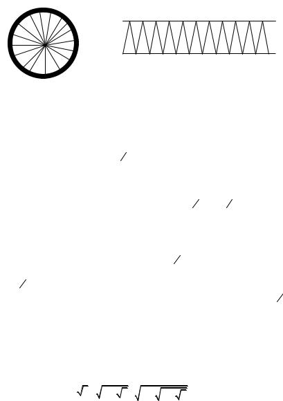
If we survey the evolution of the number concept, we see that at each crucial stage a new kind of symbolic “number” was created so as to enable a certain sort of equation to be solved. We conclude this chapter by displaying the resulting correspondence between “numbers” and equations as a scheme coreelating the type of number with the simplest equation which has that type of number as a solution.

Rational numbers:	2x = 1	Irrational numbers:		x2 = 2
Zero:	x + 1 = 1 Negative numbers:			x + 2 = 1
	Complex numbers:		x2 + 1 = 0

52

CHAPTER 3

In Chapter 8 we will discuss infinite numbers, which may be brought into the scheme as

Infinite numbers:

x + 1 = x.