Chebyshev internet

EE648 Chebyshev Filters

08/31/11

John Stensby

The Chebyshev polynomials play an important role in the theory of approximation. The

Nh-order Chebyshev polynomial can be computed by using

T (Ω) =	cos(N cos−1(Ω))	,		Ω		≤1
N						(1.1)
	cosh(N cosh−1(Ω))
=		,		Ω		>1.

The first few Chebyshev polynomials are listed in Table 1, and some are plotted on Figure 1. Using T0(Ω) = 1 and T1(Ω) = Ω, the Chebyshev polynomials may be generated recursively by using the relationship

TN+1(Ω) = 2ΩTN (Ω) −TN−1(Ω) ,

(1.2)

N ≥ 1. They satisfy the relationships:

1.For Ω ≤ 1, the polynomial magnitudes are bounded by 1, and they oscillate between ±1.

2.For Ω > 1, the polynomial magnitudes increase monotonically with Ω.

3.TN(1) = 1 for all n.

4.TN(0) = ±1 for n even and TN(0) = 0 for N odd.

5.The zero crossing of TN(Ω) occur in the interval –1 ≤ Ω ≤ 1.

N	TN(Ω)
0	1
1	Ω
2	2Ω2 – 1
3	4Ω3 - 3Ω
4	8Ω4 - 8Ω2 + 1

Table 1: Some low-order Chebyshev polynomials

Page 1 of 24

EE648 Chebyshev Filters

08/31/11

John Stensby

Chebyshev Polynomials

12

6 = n

10

Tn(ω)

4 = n

3 = n

8

6

4

2

0

	2
n	=

n =1

0.0

0.2

0.4

0.6

0.8

1.0

1.2

1.4

1.6

1.8

ω

Figure 1: Some low-order Chebyshev polynomials.

Chebyshev Low-pass Filters

There are two types of Chebyshev low-pass filters, and both are based on Chebyshev polynomials. A Type I Chebyshev low-pass filter has an all-pole transfer function. It has an equi-ripple pass band and a monotonically decreasing stop band. A Type II Chebyshev low-pass filter has both poles and zeros; its pass-band is monotonically decreasing, and its has an equirriple stop band. By allowing some ripple in the pass band or stop band magnitude response, a Chebyshev filter can achieve a “steeper” passto stop-band transition region (i.e., filter “roll-

Page 2 of 24

EE648 Chebyshev Filters

08/31/11

John Stensby

off” is faster) than can be achieved by the same order Butterworth filter.

Type I Chebyshev Low-Pass Filter

A Type I filter has the magnitude response

Ha ( jΩ)		2	=	1				,	(1.3)
					1+ε2T2	(Ω/ Ω	)
					N	p

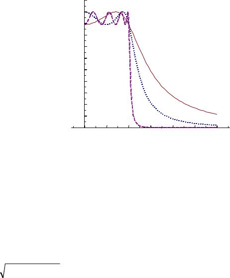
where N is the filter order, ε is a user-supplied parameter that controls the amount of pass-band ripple, and Ωp is the upper pass band edge. Figure 2 depicts the magnitude response of several Chebyshev Type 1 filters, all with the same normalized pass-band edge Ωp = 1. As order N increases, the number of pass-band ripples increases, and the “roll – off” rate increases. For N odd (alternatively, even), there are (N+1)/2 (alternatively, N/2) pass-bank peaks. As ripple parameter ε increases, the ripple amplitude and the “roll – off” rate increases.

On the interval 0 < Ω < Ωp, TN2 (Ω/ Ωp ) oscillates between 0 and 1, and this causes

Ha(Ω/Ωp) 2 to oscillate between 1 and 1/(1 + ε2), as can be seen on Figure 2. In applications, parameter ε is chosen so that the peak-to-peak value of pass-band ripple

Peak − to − Peak Passband Ripple = 1−1/ 1+ ε2 .

(1.4)

is an acceptable value. If the magnitude response is plotted on a dB scale, the pass-band ripple becomes

		1			=10Log(1+ε2 ) .
Pass −Band Ripple in dB ≡ 20Log						(1.5)
		1+ε	2
1/

In general, pass-band ripple is undesirable, but a value of 1dB or less is acceptable in most

Page 3 of 24

EE648 Chebyshev Filters

08/31/11

John Stensby

Type 1 Chebyshev Low-Pass Filter Magnitude Response

	1.1
	1.0
	0.9					Ωp = 1.0
)						Ripple = 1dB
(jΩ	0.8
a
H	0.7
	0.6
Magnitude
	0.5
	0.4
	0.3				N = 2
	0.2				N = 3
	0.1			N = 8
	0.0	0.5	1.0	1.5	2.0	2.5	3.0

Frequency Ω

Figure 2: Type I Chebyshev magnitude response with one dB of pass-band ripple

applications.

The stop-band edge, Ωs, can be specified in terms of a stop-band attenuation parameter. For Ω > Ωp, the magnitude response decreases monotonically, and stop-band edge Ωs can be specified as the frequency for which

	1		<	1	, Ω > Ωs > Ωp ,	(1.6)
2	2			A
		(Ω/ Ωp )
1+ε	TN

where A is a user-specified Stop-Band attenuation parameter. In Decibels, for Ω > Ωs, the magnitude response is down 20Log(A) dB or more from the pass band peak value.

Type I Chebyshev Low-Pass Filter Design Procedure

To start, we must have Ωp, Ωs, pass-band ripple value and the stop-band attenuation value. These are used to compute ε, N, and the pole locations for Ha(s), as outlined below.

1) Using (1.5), compute

Page 4 of 24

EE648 Chebyshev Filters

08/31/11

John Stensby

ε = 10{Pass−Band Ripple in dB}/10 −1 .

2) Compute the necessary filter order N. At Ω = Ωs, we have

1

=

1

1+ ε2T2

(Ω

s

/ Ω

p

) = A ,

2

2

(Ωs / Ωp )

A

N

1+ ε

TN

which can be solved for

T

(Ω

s

/ Ω

p

) = cosh(N cosh−1(Ω

s

/ Ω

p

)) =

A2 −1

.

N

ε2

Finally, N is the smallest positive integer for which

N ≥	cosh−1	(A2 −1) / ε2
			.
	cosh−1(Ωs / Ωp )

(1.7)

(1.8)

(1.9)

(1.10)

3) Compute the 2N poles of Ha(s)Ha(-s). The first N poles are in the left-half s-plane, and they are assigned to Ha(s). Using reasoning similar to that used in the development of the Butterworth filter, we can write

Ha (s)Ha (−s) =	1				.	(1.11)
	1+ε2T2	(s / jΩ	p	)
	N

To simplify what follows, we will use Ωp = 1 and compute the pole locations for

Page 5 of 24

EE648 Chebyshev Filters 08/31/11 John Stensby

Ha (s)Ha (−s) =	1		.	(1.12)
	1+ε2T2	(s / j)
	N

Once computed, the pole values can be scaled (multiplied) by any desired value of Ωp. From inspection of (1.12), it is clear that the poles must satisfy

T (s / j) = ± −1/ ε2	= ±j/ ε	(1.13)
N

(two cases are required here: the first where + is used and the second where − is used). Using (1.1), we formulate

	cos N cos−1(s / j) = ±j/ ε.				(1.14)
	We must solve this equation for 2N distinct roots sk, 1 ≤ k ≤ 2N. Define
	cos-1(sk/j) = αk - jβk				(1.15)
	so that (1.14) yields
	cos[N(αk - jβk ) ] = cos(Nαk )cosh(Nβk ) + jsin(Nαk )sinh(Nβk ) = ±		j		(1.16)
			ε

by using the identities cos(jx) = cosh(x) and sin(jx) = j{sinh(x)}. In (1.16), equate real and imaginary components to obtain

Page 6 of 24

EE648 Chebyshev Filters

08/31/11

John Stensby

cos(Nαk )cosh(Nβk ) = 0

(1.17)

sin(Nαk )sinh(Nβk ) = ±1ε .

Since cosh(Nβk) ≠ 0, the first of (1.17) implies that Nαk must be an odd multiple of π/2 so that

	Nαk = (2k −1)	π		αk = (2k −1)	π	, k = 1, 2, 3, ..., 2N .	(1.18)
		2			2N

The αk take on values that range from π/2N to 2π – π/2N in steps of size π/2N. Since sin(Nαk) = (-1)k-1, and the sign in the second (1.17) can be + or −, we can use

βk =	1	sinh	−1		1		(1.19)
	N				ε

(all βk are identical; the 2N distinct αk will give us our 2N roots). Now, substitute (1.18) and (1.19) into (1.15) to obtain

sk = jcos(αk − jβk ) = σk + jωk ,

(1.20)

where

π

1

−1

1

σk

= −sin (2k

−1)

sinh

sinh

ε

2N

N

(1.21)

ω

= cos

(2k −1)

π

cosh

1

sinh−1

1

,

k

ε

2N

N

1 ≤ k ≤ 2N, for the poles of Ha(s)Ha(-s). The first half of the poles, s1, s2, … , sn, are in the leftPage 7 of 24

EE648 Chebyshev Filters

08/31/11

John Stensby

half of the s-plane, while the remainder are in the right-half s-plane.

For k = 1, 2, … , 2N, the poles of Ha(s)Ha(-s) are located on an s-plane ellipse, as illustrated by Figure 3 for the case N = 4. The ellipse has major and minor axes of length

			1				−1		1
d2	= cosh					sinh			ε
			N
d	=	sinh	1			sinh−1			1		,
1									ε
			N

respectively. To see that the poles fall on an ellipse, note that

σk2 + ωk2 =1

d12 d22

									Imj
d1	=sinh 1 sinh−1 1						s1		s8
	N				ε
d2	=cosh	1	sinh	−1		1
						ε
		N
									d2
								s2
									s7

d1

Re

s3s6

(1.22)

(1.23)

s4 s5

Figure 3: S-plane ellipse detailing poles of Ha(s)Ha(-s) for a fourth-order (N = 4), Chebyshev filter with 1dB of passband ripple.

Page 8 of 24

EE648 Chebyshev Filters

08/31/11

John Stensby

for 1 ≤ k ≤ 2N.

4) Use only the left-half plane poles s1, s2, … , sN, and write down the Ωp= 1 transfer function as

		(−1)n s s		s	N
	Ha (s) = K		1 2			,	(1.24)
		(s −s1)(s	−s2 )	(s −sN )

where K is the filter DC gain. To obtain a peak pass-band gain of unity, we must use

K =	1	,	N even
	1+ε2
=	1,		N odd.

However, K can be set to any desired value, within technological constraints.

5) For a non-unity value of Ωp, the transfer function becomes

(−1)n s s

s

N

Ha (s) = K

1 2

.

s

s

s

−s

−s

2

−s

Ωp

1

Ωp

Ωp

N

(1.25)

(1.26)

Most hand calculators do not support hyperbolic trigonometry functions. It is desirable to develop non-hyperbolic-function forms for the Chebyshev filter formulas. To accomplish this,

we use

sinh

−1

(x) = ln

x

2

+1

to implement the simplification

x +

1

−1

1

1

1+ 1+ε2

sinh

=

ln

= ln( Γ) ,

(1.27)

N

N

ε

ε

Page 9 of 24

EE648 Chebyshev Filters

08/31/11

John Stensby

where Γ is defined as

1+

1/ N

1+ε2

(1.28)

Γ ≡

ε

.

In terms of parameter Γ, we can use (1.27) to write

1

−1

1

= cosh (ln(Γ)) =

eln(Γ) +e−ln(Γ)

=

Γ +1/ Γ

=

Γ2

+1

cosh

sinh

ε

2

2

2Γ

N

(1.29)

eln(Γ) −e−ln(Γ)

1

−1

1

= sinh (ln(Γ)) =

=

Γ−1/ Γ

=

Γ2

−1

sinh

sinh

ε

2

2

2Γ

.

N

Now, use (1.29) in the pole formulas (1.20) and (1.21) to obtain
		π Γ2 −1					π		Γ2 +1
sk = −sin (2k	−1)			2Γ	+ jcos (2k	−1)			2Γ	,	(1.30)
		2N					2N

1≤ k ≤ 2N, for the 2N poles of Ha(s)Ha(-s). Also, the poles are on an s-plane ellipse with major and minor axes

		1				−1		1			Γ2 +1
d2	= cosh				sinh			ε		=	2Γ
		N
											(1.31)
d	= sinh	1			sinh−1			1		= Γ2 −1 ,
1								ε			2Γ
		N

respectively.

Page 10 of 24