Bologna / 02_TCAD_laboratory_A_simulation_primer_GBB_20140326H1020

Example

M. A. Alam (2008),

"ECE 606: Principles of Semiconductor Devices,“

http://nanohub.org/resources/5749.

Italy, France, Germany and UK form our ‘system’. Italian population is the ‘quantity of interest’. Immigration/emigration in/from the other countries are our ‘processes’.

France

4

4 Italy

4

4

2 2

Germany

UK

EQUILIBRIUM

10 people going out and 10 people coming in Italy (population of Italy is “stationary”).

In addition, immigration and emigration counterbalance country-wise (each process counterbalance its opposite in each country): we are in equilibrium condition.

France 5

3 Italy

3

4

2 3

Germany

UK

STEADY STATE

10 people going out and 10 people coming in Italy (population of Italy is stationary)

But immigration and emigration process do not counterbalance countrywise: we are out-of- equilibrium.

France 2

6 Italy

1

4

5 2

Germany

UK

TRANSIENT

12 people going out and 8 people coming in Italy. Italian population is not conserved, i.e. Italian population is not stationary. In addition, immigration and emigration do not counterbalance

country-wise: we are out-of-

G. Betti Beneventi 11 equilibrium.

Outline

•Introduction

•Definition of equilibrium and out-of-equilibrium

•Static, Transient and AC simulations

 Simplify the simulation domain

•Numerical methods from a TCAD user perspective

•Meshing

•Numerical methods

•Synopsys Sentaurus TCAD Solvers

G. Betti Beneventi 12

Simulation on 1D, 2D and 3D domains (1)

•Reality is always 3D. However, some problems can be thought (approximated) as they would occur in less than 3D. This can be done when there is invariance of the problem on some directions. In other words, a dimension can be suppressed from the simulation if the physical internal properties of the simulated device would not change if the dimension itself would be made infinite. To make such approximations (not always easy to see!), an a-priori knowledge of the problem is needed.

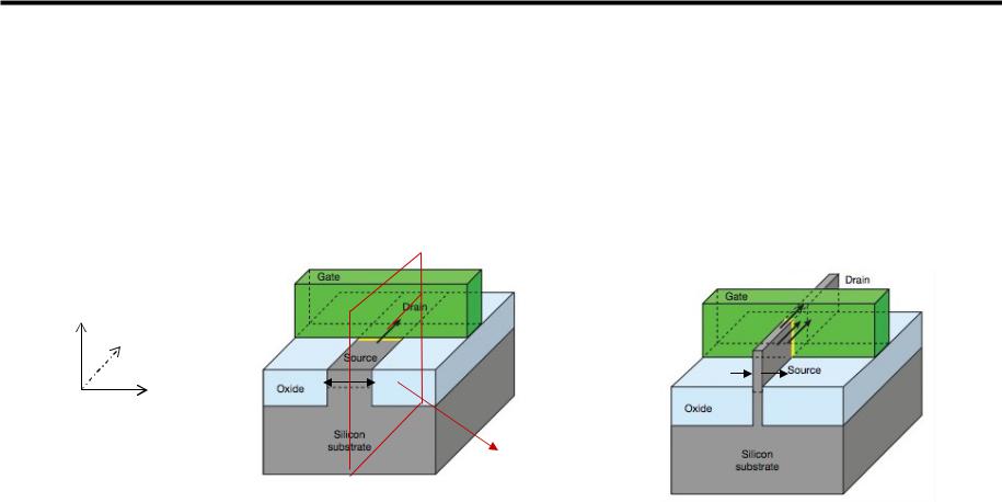
Example	Standard planar MOSFET

z

y

x	L
	2D

Possible to think about a 2D equivalent (on the yz plane) of what happens in the transistor channel. That is the device features can be thought to be invariant in the x direction (within the channel). The larger the L the better the 2D approximation.

FinFET

L

L very thin and raised source and drain. Intrinsically a 3D device, very difficult to simplify into a 2D equivalent!

G. Betti Beneventi 13

Simulation on 1D, 2D and 3D domains (2)

•The simplification of a 3D problem into 2D or even 1D, if possible, is strongly encouraged . Indeed, the simplification of the simulation domain, means a lower number of nodes in which the numerical simulation must be computed. Reducing the number of the mesh nodes decreases the computational burden and therefore the time needed for the simulation to be performed.

e.g.: same device, for 2D simulation ~ 103 nodes, for a 3D simulations ~105 nodes ~ 2 orders of magnitude of difference in the node numbers!

•One of the most frequently employed simplification is simulating a 3D device having cylindrical symmetry using a 2D domain and solving the model equations in cylindrical coordinates.

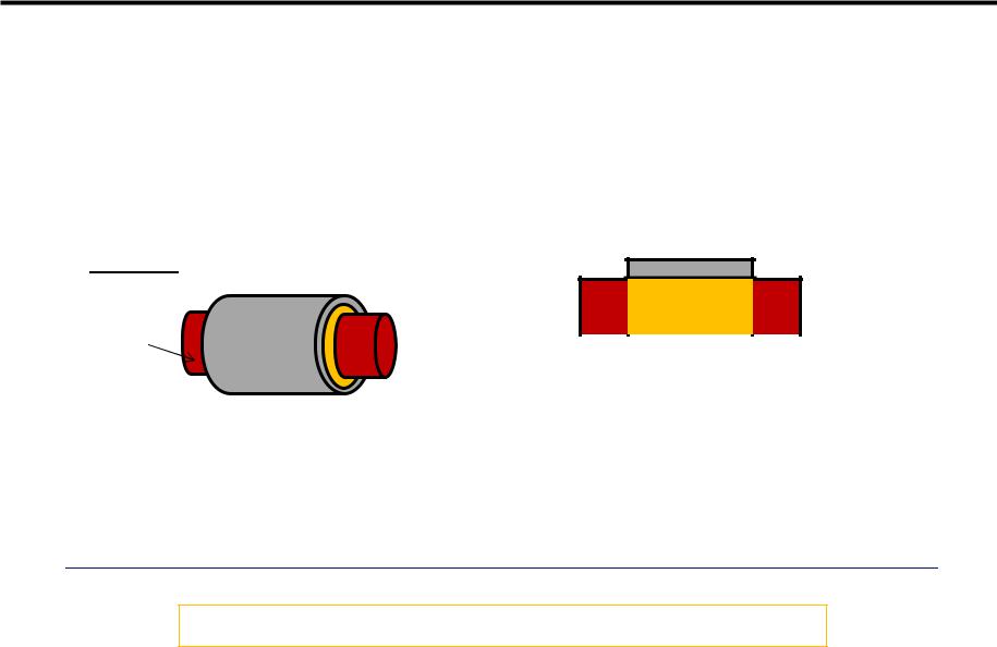
Example Nanowire (NW) MOSFET

drain

source gate equivalent 2D domain to be simulated

in cylindrical coordinates

•To simulate a 2D domain in cylindrical coordinates, the partial-differential equations must be expressed in the cylindrical coordinate system. In Sentaurus Synopsys this is accomplished by using the Cylindrical keyword in the Math section of the Sdevice input file (see later)

•Because of the simple geometry, all the devices simulated in the course need only a 2D planar (*) simulation domain.

(*)planar = Cartesian coordinates vs. cylindrical coordinates

G. Betti Beneventi 14

Outline

•Introduction

•Definition of equilibrium and out-of-equilibrium

•Static, Transient and AC simulations

•Simplify the simulation domain

Numerical methods from a TCAD user perspective

•Meshing

•Numerical methods

•Synopsys Sentaurus TCAD Solvers

G. Betti Beneventi 15

Scope

•In this tutorial we discuss the basic features of the numerical method used in TCAD Sentaurus Devices from a TCAD user perspective. The purpose of this tutorial is not describing into details the numerical methods implemented in the software, but discussing their general features, in order for the user to understand which numerical methods is most useful to be employed for a given problem and to cope with possible convergence issues.

•In general, in an iterative solution method, we start with a guess for the solution (often the zero vector) and then we successively renew this guess, getting closer to the solution at each stage. The iterations continue until the solution converges to a desired accuracy

xi –xi-1 < e, where x is the solution vector, that is the vector of the values of the problem unknowns, i is the index counting the iteration number, and e is the vector which defines the needed accuracy.

G. Betti Beneventi 16

Outline

•Introduction

•Definition of equilibrium and out-of-equilibrium

•Static, Transient and AC simulations

•Simplify the simulation domain

•Numerical methods from a TCAD user perspective

 Meshing

•Numerical methods

•Synopsys Sentaurus TCAD Solvers

G. Betti Beneventi 17

Considerations on numerical mesh (1)

•Define and effectively optimize numerical meshes in which the problem can be solved assuring convergence and, at the same time, reasonable simulation times, is a challenge. However, some general rules can be applied:

•The grid spacing must be sufficiently dense so that all the relevant features of the geometry (e.g. doping) are accurately represented.

•Points must be allocated to accurately approximate the physical quantities of interest (e.g. potentials, fields, carrier concentrations, currents).

•This means that high grid densities must be allocated in regions where the geometrical and physical quantities of interest undergo rapid changes (e.g. junctions).

•Conversely, the spacing between points could be relaxed in the areas where values are expected to stay relatively constant without adding any significant contribution to the overall error (e.g. quasi-neutral regions, deep regions inside the device). In fact, because the overall computation time depends on the total number of grid points, grid point number must be minimized for computational efficiency.

•In advanced finite-element software, as well as in Synopsys Sentaurus there are tools for automated grid generation and automatic adaptation of grids.

G. Betti Beneventi 18

Considerations on numerical mesh (2)

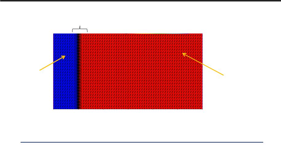
Example. Numerical grid in a pn diode

junction

p region

n region

•Once that convergence is achieved within reasonable simulation time, an operation that must always been performed prior to elaborate the results of a simulation is to check the invariance of the solution with respect to variations of the numerical mesh. That is, once a mesh has been created to assure convergence in reasonable time, try to further reduce the mesh spacing and see if the solutions does not change. If the solution does not change mesh is good !

G. Betti Beneventi 19

Outline

•Introduction

•Definition of equilibrium and out-of-equilibrium

•Static, Transient and AC simulations

•Simplify the simulation domain

•Numerical methods from a TCAD user perspective

• Meshing

 Numerical methods

• Synopsys Sentaurus TCAD Solvers

G. Betti Beneventi 20