Mini-course 1 Decision Analysis (Dr. Mariya Sodenkamp) / Class 1 / Even SWAP Operation Analysis

F P h o t o		OPERATIONAL ANALYSIS
U S A

Global Hawk

OPTION ANALYSIS:

USING THE METHOD OF EVEN SWAPS

by Dr. W.J. Hurley and Dr. W.S. Andrews

n important problem for defence planners is					To illustrate the method, we use a simple example
assessing the trade-off among decision factors				involving the selection of an Unmanned Aerial Surveillance and
(criteria)1 for competing systems. Among the				Target Acquisition System (UASTAS). A typical UASTAS
operations research tools available for such				system comprises ground stations and unmanned airframes.
analyses, Multi-Criteria Decision Analysis				Airframes are programmed to fly over forward areas of the
A(MCDA) is perhaps the most useful.				battlefield. They have extremely sophisticated on-board sensor
				systems which transmit almost-real-time information (including
In the case where a staff officer uses a MCDA technique,				video) from their field of view back to a ground station. The
say in an Options Analysis, he usually has to sell the argument				problem is to choose the preferred option given assessments
to senior decision-makers. Depending on the complexity of the				of each system on a number of important factors.
MCDA tool used, this can be a very difficult task – especially				AN EXAMPLE
if superiors are unfamiliar with the specific tool being used.
The staff officer ends up with two problems. First, he must					uppose you are a staff officer assigned to the UASTAS
convince his superiors that the technique he is using is
appropriate. Then, assuming he can do this, he must argue his			Sproject described above. You are responsible for an Options
preferred alternative within the structure of this technique. If				Analysis to determine which of four compliant off-the-shelf
his technique is complex, the first of these problems is difficult.				systems is best. These are labelled A, B, C and D. After consul-
The officer must make a decision regarding how much to				tation with fellow staffers, you arrive at the following set of
reveal about his ‘Black Box’. This almost always boils down				assessment criteria:
to a state of affairs where the officer invokes academic cant, the				•	Range: the effective range of an airframe measured in
superior does not fully understand the ‘Black Box’, and the
decision is made largely on the basis of faith and the reputation					kilometres.
of the staff officer.				•	Field of View: an aggregate measure of the range of
In this note we present a simple MCDA technique					sensors measured in square kilometres.
termed the Method of Even Swaps.2 This method arrives at a
preferred alternative through a series of simple comparisons				Dr. W.J. Hurley is a professor in the Department of Business
and judgments. It has the characteristic that most intelligent				Administration and Dr. W.S. Andrews is a professor in the Department
decision-makers can easily understand it. Moreover, it lays				of Chemistry and Chemical Engineering at the Royal Military
bare the critical assumptions that lead to a preferred alternative.				College of Canada.
Autumn 2003	●	Canadian Military Journal			43

•Response Time: the time in minutes to mission-plan and launch a back-up airframe in the event in-flight reprogramming is not possible.

•Survivability: the probability an airframe completes a mission in a defined hostile environment. (It was estimated with error by Land Operational Research Staff).

•Cost: the sum of the Procurement Cost and the discounted future costs of Operation, Personnel and Maintenance, measured in present-year dollars.

This is a fairly small set of criteria by DND Option Analysis standards. But since our purpose is simply to demonstrate how the technique works, we make no claim that these criteria are complete or consistent.

These criteria and options give rise to the following Consequences Table:

Consequences Table

System A		System B	System C	System D
RANGE	56	60	60	55
FIELD OF VIEW	1.00	1.18	1.15	1.15
RESPONSE	62	60	50	70
SURVIVABILITY	0.85	0.90	0.90	0.92
COST	52	49	42	55
Table 1

Each system is measured on each criterion. In the absence of objective data for a criterion, the decision-maker could simply rank-order the systems. That is, a ‘1’ would be assigned to the system which is best on that criterion, a ‘2’ to the second best system, and so on.

With this Consequences Table in hand, the systems are then rank-ordered on each assessment criterion:

Consequences Table (Rank-Order)

System A		System B	System C	System D
RANGE	3	1	1	4
FIELD OF VIEW	4	1	2	2
RESPONSE	3	2	1	2
SURVIVABILITY	4	2	2	1
COST	3	2	1	4
Rank Sum	17	8	7	15
Table 2

For instance, consider each system on the Range criterion. Systems B and C have the highest range and consequently each is assigned the rank 1. System C has the next highest range followed by System D. Therefore we assign a rank of 3 to System A and 4 to System D.

The bottom row of this rank-order consequences table is the sum of the column rank-orders. Clearly we would like to look at systems with low rank-order sums. In this case, Systems B and C have low rank-sums; Systems A and D have high rank-sums.

We begin pruning the Consequences Table by looking for dominated alternatives. Consider Systems A and B. Note that B has a lower rank-order for every assessment criterion. Hence A is said to be dominated by B and we can exclude System A from further consideration.

Now we examine System B and System D. System B is at least as good as System D for every assessment criterion except Survivability. Given that Survivability is measured with error and the two measures are close anyway (.90 for System B and .92 for System D), the decision is made that System B is preferred to System D. We say that System D is nearly dominated by System B and System D is eliminated.

The reduced Consequences Table is as follows:

Consequences Table

	System B	System C
RANGE	60	60
FIELD OF VIEW	1.18	1.15
RESPONSE	60	50
SURVIVABILITY	0.90	0.90
COST	49	42
Table 3

Note that these two systems have identical measures on Range and Survivability. We can now eliminate these criteria to reduce the Consequences Table to:

Consequences Table

	System B	System C
FIELD OF VIEW	1.18	1.15
RESPONSE TIME	60	50
COST	49	42
Table 4

44

Canadian Military Journal

●

Autumn 2003

Now we are in a position to do an even swap. Consider System C and ask what we are prepared to pay in dollars (Cost) to get the Field of View up to 1.18 square kilometres. Suppose we are prepared to pay an additional $2 million.3 Then, the revised Consequences Table is:

Consequences Table

	System B	System C
FIELD OF VIEW	1.18	1.15+.03
RESPONSE TIME	60	50
COST	49	42+2
Table 5

and now we can eliminate the Field of View criterion giving:

Consequences Table

	System B	System C
RESPONSE TIME	60	50
COST	49	44
Table 6

Now the decision is clear. System C has a lower Response Time and a lower Cost. Hence System C is preferred to System B, and therefore System C is the preferred option.

Note that we have arrived at the conclusion that System C is best with only one assumption: as long as we are prepared to pay something less than $7 million for a 2.6 percent increase in System C’s Field of View, System C is the best alternative.

SOME GENERAL POINTS

Suppose we define a decision path to be a sequence of dominance and even swap decisions that lead to the specification of a preferred alternative. It should be clear that, for any Consequences Table, there are a variety of paths that result in a

preferred option.

It should also be noted that we could ask a decision-maker to specify some trade-offs a priori. For instance we could ask the decisionmaker how much he is prepared to pay to get a 10 percent increase in Field of View, how much he is prepared to pay to get a 10 percent decrease in Response Time, and so

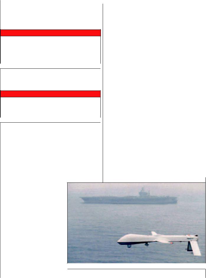
Predator

on for the other two criteria. Assuming linearity of preferences,				ANALYSIS
this would enable us to collapse the Consequences Table in a
single step. However, as the example above demonstrates,
this is not required. In that example, we required the decision-
maker only to specify a single trade-off.
In this regard, there is a common misconception about
how this method works. Some have suggested that the				OPERATIONAL
Iits origin in the rather famous		advice that Benjamin
method is faulty because it implicitly assigns equal weights
to the criteria. Of course, this is not the case. While it is true
that the Method of Even Swaps does not require us to assign
relative values to all criteria (as we have to do in just about
every other multi-criteria system), it is hardly the case that
we implicitly assess these as equally weighted.
SUMMARY
t is worth pointing out that the Method of Even Swaps has
Franklin offered Joseph Priestly:
... To get over this, my way is to divide half a sheet of
paper by a line into two columns; writing over the one
‘Pro’, and over the other ‘Con’. Then, during three or
four days’ consideration, I put down under the different
heads short hints of the different motives that at
different times occur to me, for or against the measure.
When I have thus got them
all together in one view,		“The Method of
I endeavor to estimate their		Even Swaps ... arrives
respective weights; and where
		at a preferred
I find two ones on each
side that seem equal, I strike		alternative through
them both out. If I find		a series of simple
a reason pro equal to two
		comparisons and
reasons con, equal to some
three reasons pro, I strike out		judgments.”
the five....

U S N P h o t o

Autumn 2003

●

Canadian Military Journal

45

“Our view is that the Method of Even Swaps is especially useful when a preferred option must be ‘sold’ to senior decision-makers.”

Hammond, Keeney and Raiffa have extended Franklin’s logic in a very creative way to the case where there are more than two alternatives.4

In some cases, it may well be that the Method of Even Swaps is not appropriate. In

fact, Guitouni and Martel argue that it is unlikely one MCDA technique will ever prove superior for all decisions.5 This position is certainly consistent with the large number of multi-criteria models available. While it may be true that other MCDA approaches offer better discrimination among options at the cost of complexity in some cases, our view is that the Method of Even Swaps is especially useful when a preferred option must be ‘sold’ to senior decision-makers.

S A G E M P h o t o

Sperwer

NOTES

1.	In the operations research literature,		‘criteria’	Business Review, March-April 1998, pp. 137-149
	refers to	characteristics which are important		and John S. Hammond, Ralph L. Keeney and
	to the decision-maker. For instance, if we			Howard Raiffa, Smart Choices: A Practical
	were considering tanks, the size of the gun would			Guide to Making Better Decisions, Harvard
	be a criterion. Within DND, the word ‘factor’			Business School Press, Boston, 1999.
	is used in the same sense. We use		the two 3.	The method does not require that we do an
	interchangeably throughout this paper.			even swap with dollars. We could have used the
2.	See John S. Hammond, Ralph L. Keeney			Field of View and Response Time criteria.
	and Howard Raiffa, “Even Swaps: A Rational			However, given our experience with this
	Method	for Making Trade-Offs,”	Harvard	methodology, decision-makers find it easier to
				make swaps with the Cost criterion.

4.Hammond et al, Op. Cit.

5.Adel Guitouni and Jean-Marc Martel, “Tentative Guidelines to Help Choosing an Appropriate MCDA Method,” European Journal of Operations Research 109, 1998, pp. 501-521.

The authors would like to thank LieutenantColonel (ret’d) Mike McKeown for background information and Captain Laim McGarry for very helpful comments.

46

Canadian Military Journal

●

Autumn 2003