Invitation to a Contemporary Physics (2004)

4.4. Cooling and Trapping of Atoms: Towards BEC

135

back to the ground state re-emitting a photon in the process. This finite lifetime (τ) implies a minimum energy spread (line-width Γ) for the excited state through one of Heisenberg’s uncertainty principles (Γ h/τ). Thus, the sharp line from the strict resonance condition relaxes to a broader absorption profile for the g–e transition with a peak centered at the atomic resonance νa. The resonance condition hν = Ee− Eg then need hold only to within this broader sense for a real transition (Fig. 4.3b).

And now for laser Doppler cooling. First, consider an atom placed in the beam of light from a tunable laser with both the atom and the laser at rest in the laboratory. Let the laser be red-detuned with respect to the atomic resonance, i.e., νL < νa with the amount of detuning δ = νL −νa Γ/h. We may take the laser beam to be directed along the positive x-axis, west to east, say. The response of the atom will then follow its absorption profile as the laser frequency is varied, with a maximum at the resonance, νL = νa, the center frequency.

Now let the atom move with a velocity Va directed east to west, i.e., along the negative x-axis, and, therefore, moving oppositely to the incident laser beam. The Doppler e ect now comes into play. The frequency of the laser light as seen by the moving atom will be blue-shifted closer into resonance, enhancing thereby the probability of absorption that would impart a momentum (velocity) kick directed opposite to atom’s motion. This causes slowing down, or deceleration of the atom. But what if the atom were moving west to east, i.e., in the direction of the light beam, you may ask. Well, any absorption must then speed up (accelerate) the atom eastwards. But, inasmuch as the light frequency will now be further red-detuned away from the resonance, the eastward acceleration will be relatively smaller. All we have to do now is to replace the single west to east laser beam with a pair of counterpropagating red-detuned laser beams aligned east-west. (In practice, a beam from a single laser is split in two using half-silvered mirrors, etc.) A little thought will convince you then that the atom will now be slowed down irrespective of whether it is moving eastwards or westwards, and that the retardation will be proportional to its instantaneous velocity. Next, what if the atom is moving north-south, or up-

z

y

optical molasses

x

νL < νa

Figure 4.5: Cooling of atoms in optical molasses: Three pairs of counter-propagating mutually perpendicular beams of red-detuned laser light. (Schematic).

136 Bose–Einstein Condensate: Where Many Become One and How to Get There

down, as indeed it will in a gas. Well, we simply do more of the same: three pairs of counter-propagating red-detuned laser beams aligned along the three mutually perpendicular directions will su ce — after all, any velocity can be resolved into three such orthogonal components (Fig. 4.5). This then is the Doppler cooling scheme. Inasmuch as the retarding force is proportional to the velocity but directed opposite to it, the Doppler cooling system acts as a viscous fluid — very aptly called optical molasses.

A nagging doubt, however, remains. The photon absorbed by the atom must eventually be re-emitted spontaneously, causing the atom to recoil. Will this recoil during the re-emission not undo what was done by the kick received during the absorption? Fortunately not! It turns out that the momentum kicks received from the absorption of the laser photons are highly directed, while the recoil kicks delivered at the spontaneous re-emission are totally un-directed (the spontaneous emission is a random, isotropic process). Therefore, on average, after repeated cycles of absorption and re-emission, the atom su ers a net slowing down. Thus, it is the directed kicks a priori followed by the undirected recoils a posteriori, that ultimately cause the Doppler cooling.

We conclude this section with a few general remarks that should place the phenomenon of Doppler cooling in a wider context. Thus, e.g., replacing the reddetuned (laser) photons by the blue-detuned photons will turn the Doppler cooling into Doppler heating — the atoms will be speeded up rather than slowed down! Also, the highly directed, coherent laser beams can be replaced by some other radiation environment with a general spectral distribution, and we may still have overall non-trivial Doppler e ects. (This will be, admittedly, less e ective from the point of laser cooling however.) Indeed, runaway Doppler instabilities due to nearresonant interaction between light and atoms have been considered on the grand astrophysical scales, away from the small laboratory scale setting, where an isotropic background radiation may replace our laboratory laser beams causing a redistribution of the atomic velocities — familiar here as the Compton–Getting e ect. Finally, what happens to the (kinetic) energy lost by the atoms as they slow down through Doppler cooling? Well, the mechanical (kinetic) energy of the moving atoms is converted into the electromagnetic energy of the photons. Recall that the red-detuned (low-energy) photons are blue-shifted (to higher energies) in each Doppler cooling cycle of absorption and spontaneous re-emission. There is also an overall increase in total entropy — thus, while the atoms are indeed being cooled down lowering their entropy, the directed photons of the coherent laser light are being converted into an undirected, incoherent radiation through the spontaneous re-emission with a relatively large increase in entropy.

4.5Doppler Limit and its Break-down

There is, however, a limit to the Doppler cooling. Even the slowest of atoms is forced to continually absorb and re-emit discrete photons in the presence of the

4.5. Doppler Limit and its Break-down

137

laser beams. The lowest temperature is reached when the viscous slowing down (dissipation) is o set by the random recoils (fluctuations) due to the spontaneous re-emissions. Such a connection between fluctuation and dissipation defining a temperature holds quite generally in physics. (The same e ect is responsible for the incessant zig-zag motion of a speck of dust, or mote in the air, even in the absence of any convection, as it receives kicks from the colliding molecules of air. There is a name for it: Brownian motion, first observed in 1827 by the Scottish botanist Robert Brown with plant pollen dispersed in water, and explained finally by Einstein in 1905 as due to collisions with the water molecules in thermal motion.) Ideally, the lowest temperature reached by the above Doppler cooling system (called the classical optical molasses) is TD = Γ/2kB, with optimal red-detuning νL − νa = −Γ/2. This follows from a rather interesting way of looking at things. The atom must be viewed as being in thermal equilibrium with the light it nearly resonates with. The width of the resonance ( Γ) may then be viewed as the thermal width kBT , giving a temperature TD. (This is true in general — the energy width of a Maxwellian distribution is indeed kBT . In fact, laser light of spectral line width ∆ is rightly viewed as having a temperature ∆/kB, i.e., the atom is now in thermal equilibrium with the laser light). Experimentally, however, temperatures much lower than the ideal Doppler limit (by as much as six times lower) were realized, which was a real surprise — an anti-Murphy law at work! The explanation for the breakdown of the Doppler limit lay in one of the most remarkable phenomena known in the schemes for laser cooling, namely that of Sisyphus cooling, recognized first by Claude CohenTannoudji and J. Dalibard. The e ect is too subtle and minute to be described cursorily. But then, one can not resist its beauty. Let us just get acquainted with the general idea of it.

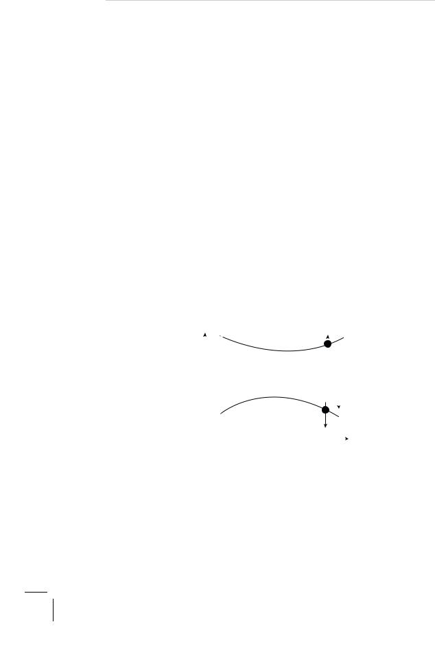
In Sisyphus cooling, we again begin with the usual scheme for the Doppler cooling involving the ground (g) and the excited (e) atomic states, but now with an additional twist, namely, that the ground state has a finer structure — it comprises two (hyperfine) sub-levels g1 and g2. Now, things are so arranged that the sub-level energies Eg1 and Eg2 vary periodically in space, along the counter-propagating laser beams that now form standing waves. The variations are, however, out of step such that when Eg1 is at a maximum, Eg2 is at minimum. These two energies act as the two possible potential-energy branches for the moving atom to lie on. Consider now an atom moving along one of these two potential-energy branches, g1 say, climbing up the potential hill as shown in Fig. 4.6, and thereby losing kinetic energy, which is now stored as potential energy. Now, matters are so arranged that as it approaches the crest of the potential hill, the energy di erence Ee − Eg1 becomes just right for it to absorb a resonant laser photon and get internally excited to the higher lying excited state (e), from which, after a short lifetime τ, it re-emits a photon spontaneously and drops back into the ground state — but this time around into the other branch (sub-level g2), which is now at its trough. With this switch thus, the atom finds itself once more at the bottom of a potential hill that must be climbed all over again as it continues to move. The energy of the spontaneously emitted photon

138 Bose–Einstein Condensate: Where Many Become One and How to Get There

g Eenergy

e

g1

g2

0

λL/4

λL/2

3λL/4

distance z

Figure 4.6: Sisyphus cooling: Atom climbs up the potential hill along g2 (or g1) converting kinetic energy into potential energy which is dissipated radiatively by optical absorption g2 (or g1) to e at the crest of g2 (or g1) followed by atom’s transfer to trough of g1 (or g2) by re-radiation e to g1 (or g2). (Schematic).

Ee − Eg2 > Ee − Eg1 , the energy of the photon absorbed. This energy di erence must equal the kinetic energy lost by the atom, and is dumped (lost) radiatively in each cycle of absorption followed by re-radiation. Hence, the Sisyphus cooling, aptly named after the Greek character who was condemned to endlessly roll his stone up the slope only to find that the slope beyond the crest was also an uphill one. Inasmuch as the Sisyphus cooling depends on the finer structure of the ground state, it is very sensitive to any external fields — even Earth’s magnetic field may have to be neutralized properly. It may be noted here that the finer sub-level energy structure, g1 and g2, of the otherwise degenerate ground state (g), which is of the essence for the Sisyphus cooling, is due to the state-dependent radiative corrections to the energy of the state — also called therefore the light-shift. (It is the change in the energy of a state due to its coupling to the photons, and depends on the intensity and polarization of the light at the place where the atom happens to be. Thus, for a standing light wave with polarization gradient, it varies periodically in space. It is a purely quantum-mechanical e ect.) The lowest temperature obtainable with Sisyphus cooling (Ts) is given by kBTs = Ω2/|δ|, where Ω (the so-called Rabi frequency) measures the strength of the light-atom dipolar coupling and δ is the detuning, assumed not too small.

The Sisyphus cooling can cool atoms below the Doppler cooling limit, TD = Γ/2kB, because now the atom does not have to equilibrate with the photon in the sense discussed earlier. The kinetic energy is being pumped out and dissipated away radiatively. There is, however, still a lower limit to Sisyphus cooling — the Recoil Limit, TR = ER/kB, where ER is the energy of the one-photon atomic recoil due to the photon momentum (h/λL) exchanged with the atom. Thus, for example, for sodium atoms (23Na), TR 2.5 microkelvin! Laser cooling below the Recoil Limit is also possible by somehow switching o the perturbing light-atom interaction — this is accomplished by pushing the atoms into the so-called Dark State. We do not, however, pursue this line of thought any further here.

4.6. Trapping of Cold Atoms: Magentic and Magneto-Optic Trap (MOT)

139

It is time now to get some feel for numbers. Consider the case of Doppler cooling for sodium atoms (23Na), where the transition involved is from the ground state (g) to the excited state (e) with the energy di erence Ee −Eg ≈ 2 electron-volt. This is the well-known yellow light from the sodium flame at the wavelength λ ≈ 589 nm. The sodium vapor emerging from a heated source (oven) is at a temperature of about 500 K, with a thermal atomic velocity of about 105 cm sec−1 (about 4000 km per hour). The momentum loss per collision (photon absorbed) h/λ, giving a velocity slow down of about 3 cm sec−1. Hence, to slow down from 105 cm sec−1 to almost zero velocity in steps of 3 cm sec−1 will require about 3 ×104 collisions. The lifetime of the excited state τ 16 ns (1 ns = 10−9 sec), giving the time required for the Doppler cooling to be 2nτ 1 ms (1 ms = 10−3 sec). The stopping distance is then about 50 cm. This amounts to an acceleration (actually deceleration) 105 × Earth’s gravity! Also, the Doppler limit TD works out to be 240 µK. As for lasers, typically, the laser power for optical molasses is 10 mW, with a bandwidth of 1 MHz and beamwidth of 2 mm radius. It is interesting to note that Doppler cooling is quite insensitive to laser power. Sisyphus cooling, however, depends strongly on the power of the laser through Ω.

4.6Trapping of Cold Atoms: Magentic and Magneto-Optic Trap (MOT)

A gas of atoms, no matter how cold, must be trapped spatially for a time long enough to be probed experimentally, or else the atoms will disperse, and most certainly fall freely under Earth’s gravity and get lost. Just as laser cooling involved confinement in velocity space centered about the zero of velocity throug the velocity-dependent forces, trapping involves confinement in the positional space centered at the origin through position-dependent forces. Such a force can derive naturally from the gradient of the potential energy of the atom placed in a suitably inhomogeneous electromagnetic field to which the atom couples. Thus, for a neutral atom one can make use of the fact that the atom may have a permanent magnetic dipole moment (µ), which when placed in a magnetic field B(x) has a potential energy −µ · B(x). (This is what makes a floating bar magnet, or the needle of a magnetic compass point due north in Earth’s magnetic field.) The same is true of alkali atoms, e.g., the sodium atom (23Na), that has an unpaired electron spin which exhibits an elementary magnetic dipole of moment µ (the Bohr Magneton) associated with its unpaired spin (with µ antiparallel to the spin). The two possible orientations of the spin, parallel and antiparallel to B di er in energy by 2µB(x). Such a splitting, or the shift of an energy level is called the Zeeman e ect. It acts on both the spin and the orbital angular momentum, with di erent strengths though. In an inhomogeneous field B(x), the potential energy is then position dependent. It has a minimum for B(x) = 0, with the magnetic moment µ antiparallel to B(x). An

140 Bose–Einstein Condensate: Where Many Become One and How to Get There

I

B

I

Figure 4.7: The quadrupolar magnetic field generated by coaxial anti-Helmholtz coils carrying oppositely directed electric currents. The magnetic field is zero at the mid-point. (Schematic).

atom with such a spin orientation seeks out the lowest field and tends to sit at the minimum of B(x). Such an inhomogeneous magnetic field can be conveniently generated with the help of two co-axial coils carrying electric currents in the opposite sense (the anti-Helmholtz coils). The resulting quadrupolar magnetic field has a zero at the mid-point on the axis as shown in Fig. 4.7. This is the canonical quadrupolar magnetic trap. The magnetic field gradient is typically 10 gauss cm−1 over a trap size 1 cm across. The trap potential is 10 mK deep in temperature units. (Room temperature of 300 K corresponds to 1/40 eV.) The lifetime of the trapped atom before it gets ejected by collisions is 100 sec at a pressure of 10−10 torr (1 atmosphere = 760 torr, 1 torr = 1 mm of Hg).

This purely magnetic trap can be integrated intelligently into the laser Doppler cooling arrangement discussed earlier. The result is a Magneto-Optic Trap (MOT), which has now become a workhorse for all BEC work. Just as laser cooling is a forced confinement of an atom in momentum (velocity) space towards the zero of momentum, magnetic trapping is a forced confinement of an atom in positional space towards the origin. The Magneto-Optic Trap (MOT) combines the two in a kind of phase-space confinement towards the zero of the velocity as well as of the position. In laser cooling we exploit the velocity-dependent Doppler shift of the light from a red-detuned laser into or o the atomic resonance. In a MOT we exploit additionally the position-dependent magnetic Zeeman shift of the atomic levels into or o the resonance with the red-detuned laser light. In all cases it can be so arranged that we have a selective and adaptive approach towards the zero of velocity and of position. Such a MOT can produce a cold cloud at about 10 µK with 1011 atoms per cm3 corresponding to a phase-space density of about 10−5, which is still far too small for BEC to occur. The cold atoms are huddled in a volume0.5 mm3 at the center of the MOT, which is about 1 cm across.

It is to be noted here that unlike the case of a purely magnetic confinement, the confining force in a MOT originates from the scattering of light involving

4.7. Evaporative Cooling			141
(a) mJ		energy
–1
0			J = 1
1	νL	σ–
σ+			J = 0
0
(b)
		σ–
I		Z	σ–
		Y
σ+		X	σ–

σ+

σ+

I

Figure 4.8: (a) Magneto-Optic Trap combining trapping (position-dependent scattering forces due to tuning by inhomogeneous Zeeman shift) and cooling, in one dimension. (b) Threedimensional MOT. (Schematic).

near-resonant absorption and re-emission — hence called the scattering (or the spontaneous) force. It is just that the condition for the resonance is made position dependent.

In Fig. 4.8a, the basic idea of a MOT is illustrated for the case of a onedimensional geometry, while Fig. 4.8b shows the schematic of a three-dimensional MOT. Because the underlying trapping mechanism in the MOT involves the Zeeman e ect, it is also referred to as the ZOT (Zeeman Shift Optical Trap). The symbols σ+, σ− here denote the circular polarization states of the light beams chosen so as to cause the atomic transitions selectively between the Zeeman-split and -shifted levels.

4.7 Evaporative Cooling: Down to the Nanokelvins

A cold atomic cloud trapped in a MOT and cooled to a few microkelvins is still a factor of 1000 away from (hotter than) the gaseous BEC that demands nanokelvins. This ultimate stage of cooling from microkelvins to nanokelvins — the last mile if you like — involves the simplest of physics, namely that of cooling by forced evaporation! Here a relatively small minority of energetic molecules with relatively large, above-average kinetic energy per capita, are allowed to escape over the potential barrier out of the trap, leaving behind the majority in the trap to settle down (re-equilibrate) to a lower average kinetic energy per capita, that is to a lower temperature. This is, of course, precisely what happens to a steaming cup of hot tea in an insulating styrofoam left out in the open. It cools mostly by evaporation, the barrier being the work function — the minimum kinetic energy needed to escape

142 Bose–Einstein Condensate: Where Many Become One and How to Get There

from the bulk liquid. The point to note here is that the amount of kinetic energy removed, or the cooling e ected, is greatly out of proportion to the mass of the liquid lost by evaporation; a mere 2% loss of molecules can cool the cup of tea by about 20%, i.e., from about 370 K to 300 K (room temperature) in a short interval of time. The e ect can be further enhanced by resorting to forced evaporation, i.e., by lowering the barrier to be overcome for the great escape. The evaporative cooling is ultimately traceable to the fact that the atoms in the fluid do not all have the same kinetic energy, or speed. There is a broad thermal distribution — the Maxwellian velocity distribution — that has a tail of very high-speed molecules that, though small in number, can and do escape over the barrier carrying away a disproportionately large amount of the energy. What is crucial, however, for evaporative cooling is the fast process of re-equilibration of the remaining molecules in the trap. This requires some inter-particle interaction which is otherwise inimical to an ideal BEC, as we have argued earlier. This calls for a compromise.

For evaporative cooling it is necessary to switch o all perturbing lasers of the MOT leaving only the confining (trapping) magnetic field on. This, in general, is the loading of a purely magnetic trap with the cold atoms from a MOT, and has been variously achieved. Through some suitable optical pumping it is so arranged that all atoms are put in the same state of the spin, with the magnetic moment (spin) antiparallel (parallel) to the trap magnetic field. As discussed earlier, the atoms with their magnetic moments aligned antiparallel to the magnetic field seek the weak field and are thus attracted towards the center of the trap. The kinetically energetic among them, however, climb up the potential barrier towards the edge of the trap as shown in Fig. 4.9. Now, the trick is to apply a radio-frequency (rf) field of the right intensity, duration and of a frequency resonant with the local Zeeman

Zeeman potential energy U(x)

U(x) = – µ · B(x)			hν

position x

Figure 4.9: Schematic of forced evaporative cooling in a magnetic trap using inhomogeneous Zeeman shift. The upper (lower) potential energy curve is for atomic spin parallel (antiparallel) to local magnetic field and has minimum (maximum) at center. Spin-flip caused by resonant rf field inverts potential upside down forcing energetic atoms nearer edge to fall o out of trap. Remaining slow moving atoms re-equilibrate to lower temperatures. Hence, forced evaporative cooling.

4.7. Evaporative Cooling

143

energy-splitting 2µB(x) so as to flip the atomic spin. This spin-flip inverts the potential barrier as seen by the atom upside down, and the energetic atoms simply fall o the edge of the trap-potential barrier, now becoming downhill. Tuning the radio frequency (rf) progressively downwards, we can e ectively move the surface- of-escape-by-spin-flip radially inward, thereby slicing o layers of atoms of lower and lower kinetic energy towards the center of the trap. One very aptly speaks of an rf-scalpel here! The gas of remaining atoms now accumulates near the center of the trap, somewhat depleted but rendered much colder and denser — possibly about 107 atoms at 1012 cm−3, huddled together in a volume 10 µm across at the center of the magnetic trap 1 cm across, and at an ultra-cold temperature of20 nanokelvins! Thus, we will have reached the coldest spot in the universe! The entire evaporative cooling cycle lasts the time scale of seconds or minutes.

It is implicit here that the magnetic moment (or the spin) of the moving atom precesses (as a spinning top) fast enough to follow the spatially varying magnetic field so as to remain locally aligned with it — actually antiparallel to it in this case. Inasmuch as the angular speed of spin precision (2µB(x)/ ) is proportional to the magnitude of the local magnetic field, this adiabatic condition must break down at and about the trap center, where the magnetic field has a pointed zero, across which the field changes its direction very rapidly. Nothing then energetically prevents the electron spin of the moving atom from flipping its direction relative to the local magnetic field vector, and, therefore, the atom from getting lost through this hole in the magnetic trap. This kind of spin flip at the zero of the magnetic field is a subtle e ect. It has a name: the Majorana Spin-Flip, said in deep voice. It must be avoided for a magnetic trap to act as a trap. A rather clever solution to this problem turned out to be just this: jiggle the pointed zero by the application of a suitable time-varying magnetic field and thus smoothen it out into a time-averaged rounded minimum. This finessing is aptly called a TOP (Time-averaged Orbiting Potential) that does plug this hole in the trap.

Nature uses evaporative cooling on all scales — we have mentioned the humble cup of hot tea as an example on the scale of centimetres, and the not so humble MOT on the scale of millimetres. But, we have evaporative cooling the scale of kilo-parsecs too (1 parsec 3.3 light years). This happens in the globular clusters of stars, where the highly energetic stars get kicked out of the gravitational barrier leaving behind a more compact cluster of less energetic stars. (In a lighter vein, the so-called Brain Drain of the Third World may well be viewed as an evaporative intellectual cooling: emigration of the higher-than-average qualified elite leading to the lowering of the average (intellectual) temperature of the population which is left behind). It seems that Nature truly has no architectural excess — it repeats the same design again and again, only the contexts and the scales may vary, and be vastly di erent!

144 Bose–Einstein Condensate: Where Many Become One and How to Get There

4.8 BEC Finally: But How Do We Know?

That is the question! There is no thermometer to tell nanokelvins anyway. Once again we have to fall back on light: this time to visualize the condensate, its distribution in velocity and position — its phase-space profile in fact — and to, therefore, indirectly act as a contactless thermometer. For this, all we have to do is to switch o the magnetic confinement too and let the ultra-cold cloud of atoms fall freely under Earth’s gravity. Once set free, the atomic cloud expands as it falls. As a result, the velocities translate into distances. In fact, for a parabolic trap the velocity distribution is the same as the spatial distribution, properly scaled. Also, the expanding cloud can be imaged by laser light which is tuned so as to be absorbed resonantly by the atoms, casting thus a shadow on a camera (the so-called Charge Coupled Device, or the CCD camera now in common use). At resonance, the cloud is almost opaque (i.e., optically thick) at the BEC phase-space density (ρ ≈ 1) and the light can hardly penetrate beyond a depth wavelength of light. But an expanded cloud is rarer and lets some light pass through, and, therfore, casts a shadow on the CCD camera whose shade (dark or grey) then depends on the column density of the cloud traversed by the laser beam. These facts together with the time of flight (TOF) allow us to essentially re-construct the velocity distribution in the cloud at di erent stages of evaporative cooling (i.e., at di erent temperatures). Typically, the BEC which is initially about 10 µm across expands to about 200 µm across in about 40 ms of the time of flight.

In Fig. 4.10, we show schematically a cross-section of the velocity (x-component, say) distribution as it evolves with cooling to lower temperatures. At relatively higher temperature, we have the well-known Maxwellian velocity distribution with its single broad Gaussian hump centred at the zero of velocity. This is the thermal cloud. As we cool down just below TBEC, a qualitative change makes appearance.

) x (vf

functiondistribution

	(a)			T< T	(b)				(c)
T > T	BEC				BEC					T<<T
				~						BEC
			)				)
			x					x
			f(v				f(v

0	vx	0	vx	0	vx
velocity		velocity		velocity

Figure 4.10: Section of distribution of ultra-cold trapped atoms imaged by expansion method:

(a) For T > TBEC showing Maxwellian thermal distribution. (b) T TBEC showing central spike of BEC emerging out of thermal Maxwellian background hump. (c) Only central spike representing fully formed Bose–Einstein Condensate (BEC). Not shown is elliptical cross-section of spike indicating anisotropy of velocity distribution in BEC in contrast with circular cross-section, or isotropy, of classical thermal background. (Schematic).