Ronald H. Dieck. "Measurement Accuracy."

Copyright 2000 CRC Press LLC. <http://www.engnetbase.com>.

Measurement Accuracy

4.1Error: The Normal Distribution and the Uniform

Distribution

Uncertainty (Accuracy)

4.2Measurement Uncertainty Model

Purpose • Classifying Error and Uncertainty Sources • ISO

Classifications • Engineering Classification • Random •

Systematic • Symmetrical Systematic Uncertainties

	4.3	Calculation of Total Uncertainty
		ISO Total (Expanded) Uncertainty • Engineering System Total
Ronald H. Dieck		Uncertainty • High Degrees of Freedom Approximation •
		Calculation Example
Pratt & Whitney	4.4	Summary

All test measurements are taken so that data may be acquired that are useful in decision making. No tests are run and no measurements made when the “answer” is already known. For data to be useful, it is necessary that their measurement errors be small in comparison to the changes or effect under evaluation. Measurement error is unknown and unknowable. This chapter addresses the techniques used to estimate, with some confidence, the expected limits of the measurement errors.

4.1Error: The Normal Distribution and the Uniform Distribution

Error is defined as the difference between the measured value and the true value of the meaurand [1]. That is,

	E = (measured)− (true)	(4.1)
where E	= the measurement error
(measured)	= the value obtained by a measurement
(true)	= the true value of the measurand

It is only possible to estimate, with some confidence, the expected limits of error. The most common method for estimating those limits is to use the normal distribution [2]. It is

Y =	1		−	1	(X −μ)2	σ2
		e	2			(4.2)

σ 2π

© 1999 by CRC Press LLC

FIGURE 4.1

where X = the input variable, here the value obtained by a measurement µ = the average of the population of the X variable

σ = the standard deviation of the population, expressed as:

å(Xi − μ)2
n
σ = i=1	(4.3)

n

where Xi = the ith X measurement

n = the number of data points measured from the population

Typically, neither n, µ, nor σ are known.

Figure 4.1 illustrates this distribution. Here, for an infinite population (N = ∞), the standard deviation, σ, would be used to estimate the expected limits of a particular error with some confidence. That is, the average, plus or minus 2σ divided by the square root of the number of data points, would contain the true average, µ, 95% of the time.

However, in test measurements, one typically cannot sample the entire population and must make do with a sample of N data points. The sample standard deviation, SX, is then used to estimate σX, the expected limits of a particular error. (That sample standard deviation divided by the square root of the number of data points is the starting point for the confidence interval estimate on µ.) For a large dataset (defined as having 30 or more degrees of freedom), plus or minus 2SX divided by the square root of the number of data points in the reported average, M, would contain the true average, µ, 95% of the time. That SX divided by the square root of the number of data points in the reported average is called the standard deviation of the average and is written as:

where SX–

S– X

X

			N	(Xi −		)2
			å		X
		=					M = SX M
S			i=1					(4.4)
	X
				N −1

=the standard deviation of the average; the sample standard deviation of the data divided by the square root of M

=the sample standard deviation

=the sample average, that is,

© 1999 by CRC Press LLC

				FIGURE 4.2
		M	(Xi N )
–		å
X	=			(4.5)

	i=1
X	= the ith data point used to calculate the sample standard deviation and the average,
i
	from the data
N	= the number of data points used to calculate the standard deviation
(N – 1) = the degrees of freedom of S		and S–
	X	X
M	= the number of data points in the reported average test result

–

X,

Note in Equation 4.4 that N does not necessarily equal M . It is possible to obtain SX from historical data with many degrees of freedom ([N – 1] greater than 30) and to run the test only M times. The test result,

or average, would therefore be based on M measurements, and the standard deviation of the average

– –

would still be calculated with Equation 4.4. In that case, there would be two averages, X. One X would

–

be from the historical data used to calculate the sample standard deviation, and the other X, the average test result for M measurements.

Note that the sample standard deviation, SX, is simply:

	N	(Xi −		)2
	å		X
SX =
	i=1				(4.6)
		N −1

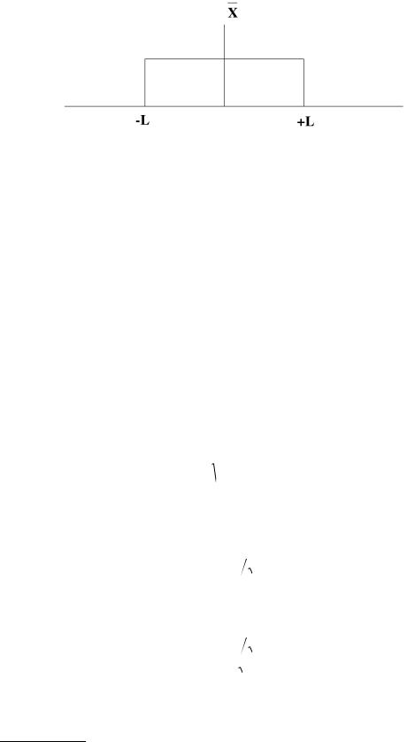
In some cases, a particular error distribution may be assumed or known to be a uniform or rectangular distribution, Figure 4.2, instead of a normal distribution. For those cases, the sample standard deviation of the data is calculated as:

SX = L 3

(4.7)

where L = the plus/minus limits of the uniform distribution for a particular error [3]. For those cases, the standard deviation of the average is written as:

S

=

L 3

(4.8)

X

M

© 1999 by CRC Press LLC