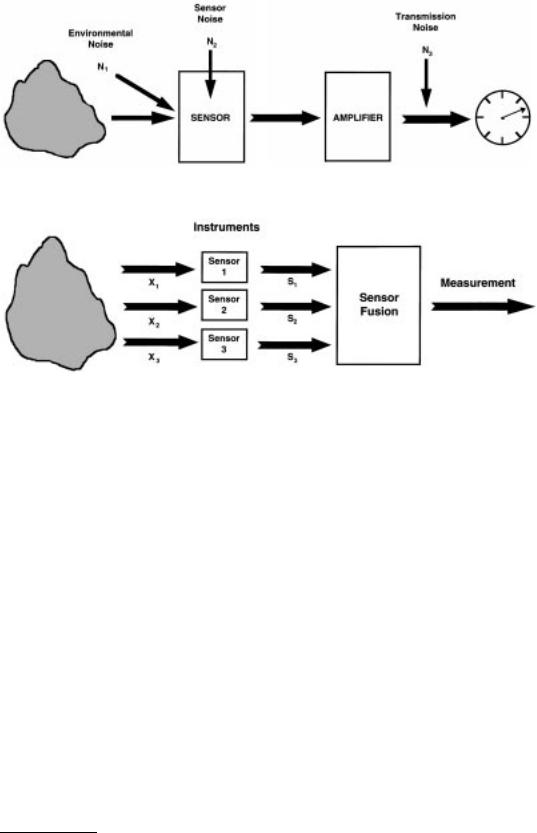
FIGURE 1.8 Instrument model with noise sources.

FIGURE 1.9 Example of sensor fusion.

Random error generating noise can also be introduced at each stage in the measurement process, as shown schematically in Figure 1.8. Random interfering inputs will result in noise from the measurement environment N1 that are introduced before the sensor, as shown in the figure. An example would be background noise received by a microphone. Sensor noise N2 can also be introduced within the sensor. An example of this would be thermal noise within a sensitive transducer, such as an infrared sensor. Random motion of electrons, due to temperature, appear as voltage signals, which are apparently due to the high sensitivity of the device. For very sensitive measurements with transducers of this type (e.g., infrared detectors), it is common to cool the detector to minimize this noise source.

Noise N3 can also be introduced in the transmission path between the transducer and the amplifier. A common example of transmission noise in the U.S. is 60 Hz interference from the electric power grid that is introduced if the transmission path is not well grounded, or if an inadvertent electric grand loop causes the wiring to act as an antenna.

It is important to note that the noise will be amplified along with the signal as it passes through the amplifier in Figure 1.8. As a consequence, the figure of merit when analyzing noise is not the level of the combined noise sources, but the signal to noise ratio (SNR), defined as the ratio of the signal power to the power in the combined noise sources. It is common to report SNR in decibel units.

The SNR is ideally much greater than 1 (0 dB). However, it is sometimes possible to interpret a signal that is lower than the noise level if some identifying characteristics of that signal are known and sufficient signal processing power is available. The human ability to hear a voice in a loud noise environment is an example of this signal processing capability.

Sensor Fusion

The process of sensor fusion is modeled in Figure 1.9. In this case, two or more sensors are used to observe the environment and their output signals are combined in some manner (typically in a processor) to

© 1999 by CRC Press LLC

provide a single enhanced measurement. This process frequently allows measurement of phenomena that would otherwise be unobservable. One simple example is thermal compensation of a transducer where a measurement of temperature is made and used to correct the transducer output for modifying effects of temperature on the transducer calibration. Other more sophisticated sensor fusion applications range to image synthesis where radar, optical, and infrared images can be combined into a single enhanced image.

Estimation

With the use of computational power, it is often possible to improve the accuracy of a poor quality measurement through the use of estimation techniques. These methods range from simple averaging or low-pass filtering to cancel out random fluctuating errors to more sophisticated techniques such as Wiener or Kalman filtering and model-based estimation techniques. The increasing capability and lowering cost of computation makes it increasingly attractive to use lower performance sensors with more sophisticated estimation techniques in many applications.

© 1999 by CRC Press LLC