Vector space

§ 1

One of the fundamental concepts of algebra is that^71,1 of vactor space: A vector space P is a k-liner set of elements, called vectors; i. e. a domian in which addition of vectors

46

47

Thе identical mapping X -»■ X is represented by the unit matrix

and multiplication of a vector by a number in ft are the permis­sible operations, satistyingg the well-known rules n vectors e_b ..., e„ form a coordinate system or a basis if they are linearly independent, while еnlargement of the sequence by any further vector world destroy this independence. Under these assumptions every vector X is uniquely expressible in

the form

(1)

where the numbers x_t are the «components» of X., The number n, which does not depend on the choice of the coordinate sys­tem is called the dimensionaility of the vector space P or the order of the linear set P. Transition to another coor­dinate system e₁, ..., e„ is effected by a nnon-sngular linear Transformation A as described by the matrix ||a_lk ||in the folio, wing manner: '

(2)

A non-singular matrix A — ||a,_k || is one whose determinant, det A or | A |, is different from 0; the inverse transformation A^-1 sends the column of n numbers x' back into the column x. On writingthe components in a column (matrix of n rows and one column), we can express (2) by the abbreviation

(3) x = Ax'

in terms of matrix calculus.

There is another interpetation of this, or rather of the modified equation x' — Ax, to the effect that it describes a linear mapping X ->- X' of P upon itself in terms of a fixed coordinate system. In that case we need not suppose A to be non-singular. A mapping X -» X' carrying each vector X into a vector X' is linear if it sends

X + n into X' + n' and aX into aX' (a any number in k). If such a correspondence changes the basic vector e_t of our coordinate system into

it will carry

When we express a given linear mapping X -» X', (4), in another coordinate system in which the vector x has the components у given by

(5)

U being the non-singular transformation matrix", the result will be

as one readily derives from (5) combined with

Hence the matrix A changes into U^-1 AU which arises from A, as we shall say, by «transformation with U». Therefore the characteristic polynomial

of the indeterminate X is independent of the coordinate system.

Obligatory Words and Word Combinations

vector space, permissible (a), coordinate system, enlarge (v), destroy (v), component (n), dimensionality (n), transition (n), non-singular (a), non-singular matrix, determinant (n), row (n), modify (v), to-the effect that, unit matrix.

§2

A linear form f (X) depending on an argument vector X may be defined without reference to a coordinate system by the functional properties: f (X + X') = f (X) + f (X'), f (aX) = a ■ f (X) (a. a number).

Its expression in terms of a coordinate system will be a linear form of the components x, of X in the algebraic sense:

49

with constant coefficients a,. Hence we know what a multi

linear form f (X g) is, depending on r argument vector.

X, ..., g. By the identification X = n = • • • = g it leads to a form f (X) of degree r of a single argument vector X. In the same manner f (X) arises from each of the forms sf (X, ..., .'

into which f (X g) changes by a permutation s of its,

arguments X, n, ..., g, and hence in particular from thesyrrt metric form

the sum here extends to all r\ permutations s. It is much easier to describe what a form of degree r is in a manner independenl of the coordinate system, by passing through the correspond ing multilinear forms. The definition of the polarized form by means of the expansion of f (X + t •n) in terms of the parameter t shows that the polar process is invariant under any change of coordinates. A natural generalization is the study of forms f (X, n, ...) depending on various argument

vectors X, n, ... with pre-assigned degrees m, v When

we stick to the algebraic model of vector space our independent definitions prove that a form f ((x)) = f (x_t ... x„) of degree changes into a similar form by any linear transformation (3); and the same is true of a form depending on various rows each of which undergoes the same transformation (3) as x. Within the n-dimensional vector space P there may be defined'¹ an m — dimensional linear subspace P_t (m < =n), A coordinate system e₁ ... e_m in Р_г can be supplemented by

я — m further vectors e_m+1 e_n to form a basis in P. Willi

respect to this basis adapted to P₁ the vectors x in P₁ are those ⁷⁵'^г whose last n — m components vanish: x — (x_v . . . , x_m, 0 0).

Hence the universal algebraic model for this situation is described thus: the vectors in P are the n-uples (x₁ ... x₁), the vectors of the subspace P_t are the n-uples of the particular form (x₁ ... x_m, 0 ... 0). P mod P₁is the (n — m)-dimensional vector space into which P turns if oneⁿ'⁶ identifies any two vectors X and X which are congruent modulo P_lt i. e. whse* difference lies in P₁

P is decomposed into two linear subspaces

P = P, + P, if each vector X splits into a sum X₁ + X₂ of a vector X₁

£0

p₁ and X₂ in P_s in unambiguous fashion. Uniqueness is assured if'the only decomposition of 0:

0 = X_l + X₂ (X, in P„ X₂ in /y

is 0 + 0, or if the two spaces are linearly independent (have no common vector except 0). A basis for P_l together with a basis for P₂ forms a coordinate system for the whole space (adaptation of the coordinates to a given decomposition); hence the sum of the dimensionalities n_х +n_а of P₁ and P_t equals n. Relative to the adapted coordinate system, the vectors of P_t and Р_г have the form

(x, ... x„„ 0 ... 0), (0 ... 0, x_n+1, .. . x„).

The word «sum» is occasionally used (but never the word «de­composition») even if unicity or linear independence does not prevail. The process of summation of (independent) parts may easily be extended to more than two summands:

P =P₁ + • • ■ + P,\ X = Xj+...+X„ X_a in P_a;

independence meaning that 0 + • • ■ + 0 is the only decompo­sition of 0 into components lying in the subspaces P_a.

Obligatory Words and Word Combinations

linear form, argument vector, without reference to, functio­nal (a), multilinear (a), identification (n), permutation (n), extend (v), polarize (v), expansion (n), parameter (n), invari­ant (a), undergo (v), n-dimensional (a), supplement (v), fa­shion (n), uniqueness (n), relative (a), occasionally (adv), prevail (v), summation (n), summand (n).

§3

wherer the matrix Ai of degree m is that⁷⁵'' induced by A in thesubspace, while A₂ may be interpreted as the corresponding

51

in case a linear mapping A carries every vector in the subspace P_t into a vector of the same subspace, we call P_х invariant under A, and the mapping A of P, upon itself is called the transformation «induced» in P_t by A. If the coor­dinate system is adapted to the subspace P, the matrix A has the form (6),

transformation of the «projected» space P mod P,. In case P breaks up into two subspaces P_t + P₂ both invariant under A, the matrix A has the form (7) in terms of a basis of P adapted to that decomposition.

One knows how matrices of a given degree m may be added, multiplied by numbers and among each other; the multiplication is associative but not commutative. The trans, posed matrix of A = || a,_k || shall⁴ be denoted by

It is the matrix of the substitution

where g denotes a row of numbers (|_t £„). A column x

of n numbers may be called a covariant, a row g a contrava-riant vector. From them we may form the product

which is a one-rowed square matrix or a number. If under the influence of transition to a new coordinate system the ,x undergo a non-singular transformation x = Uy, the g shall be subjected to the contragredient transformation

so that Ex remains unchanged:

We consider covariant and contravariant vectors as vectors in two different «dual» spaces P and P*. A change of coordi­nates in one shall be automatically connected with the contragredient change in the other space, so that the product lx has an invariant significance. The mapping x ->■ x' = Ax is in invariant manner tied up with the mapping g ->> g' = gA in the dual space:

i. e. the product of I' with x equals the product of g with the image x' of x.

Obligatory Words and Word Combinations

in case, induce (v), interpret (v), break up (v), transpose (v), covariant (contravariant) vector, contragredient (a), dual (a), image (n).

52

*⁴

An orthogonal transformation (4) is one leaving inva­riant the quadratic form

This amounts to the equation

(6)

for A, from which follows at once

(7)

sjnce the relation of a matrix A and its inverse A~' is mutual.. Another way of putting it is to say that an orthogonal mat­rix is identical with its contragredient. As for the determinant,, it follows from (6) that its square = 1, hence

According to these two cases one^76,6 speaks of a proper or an improper¹ orthogonal transformation.

Let A_tk be (—1)^i-k times the determinant of the matrix A after the i'^h row and k^,h column have been cancelled. The familiar identities

^r=1

according as i = k or i <> k, show that for a non-singular A the quotient A_kl/det A is the (ik) — element of the inverse ^A-l; hence the contragredient matrix is

we therefore have

may be denoted by

according as Л is a proper' or an improper orthogonal trans­formation. The minor

TEXT THIRTEEN

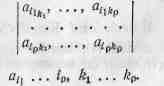
In the theory of determinants one proves the following indenti. ties between the minors of |a,₄| and those of )4,J:

(9) A_n ... if,, k_t... kg, = (det Af~^l. a₄... т„, x_x... x„. Here p + a = n and

h ■ •"• 'Л ... to, ftj ... кц^ ... Ka stand for two even permutations of the figures 1, 2, ..., n. In particular

det (A_it) = (det (a«))»-¹. For an orthogonal matrix A we combine (9) and (8) and find:

(10) a_t.,,../«, ^ ... £_p = ± a,, ... т„, x_t ... x₀,

#ie wpper sign holding again for the proper and the lower for the improper transformations". These simple formal relations will later on be useful.

Everybody is familiar with the part the orthogonal trans­formations play in the most fundamental — the Euclidean — geometry, where, after the choice of the unit of length, foot or meter, each vector JC has a certain length, the square of which is given by a positive definite quadratic form (XX) in X. The corresponding symmetric bilinear form is the scalar product (Xti). The condition (Xri) = 0 means that X and n are perpendicular. An orthogonal or Cartesian coordinate system e_v ..., e„ is one⁷⁶'" in which (XX) has the normal form

(XX) = дг? + • • • +4, or, in other words, one such that

e_te_k = 6,_k. All Cartesian coordinate systems are equivalent in Euclidean geometry; the transition from one Cartesian coordinate system to another is accomplished by means of an orthogonal trans­formation; according as it is proper or improper the two systems are of equal or opposite «orientation». A linear mapping X -» ->- X'= At leaving unchanged the lengths of vectors is expressed in terms of a Cartesian coordinate system by an orthogonal matrix A; in case A be'¹ proper we have to do with a «rotation».

Obligatory Words and Word Combinations

orthogonal (a), mutual (a), familiar (a), minor (n), identi­ty (n), stand for (v), scalar (a), accomplish (v), orientation (n), rotation (n).

SOME CONCEPTS OF THE THEORY OF CURVES

§1 Q

W/e^ can think of curves in space as paths of a point in пкЖоп: The rectangular coordinates (x, у, г) of the^point can then be expressed³as functions of a parameter и inside a certain closed interval:

(la) x = л:(и) ^=j/(«), г = г(я); ы₁<и<и_г.

It is ofjen convenient to think,of и as the time, but this is not песейагу, sincf^ we can pass^from one parameter to- another by a substitution и =»'J (%) without changing™ the curve itself. We select the coordinate axes in such a way that the sense OX -> 0У -»- OZ is that^,5,e of a right-handed screw. We also denote (л:, у, г) by (x_lt x., x₃) or for short⁸³, x_lt i = 1, 2, 3. The equation of the curve then takes the form | (lb) x_t = ДГ((И); %<«<«„.

We use the notation P (x_t) to indicate a point with coordi­nates x_t.

Example. Straight line, A straight line in space can be given by the equation

(2) x, = a_t + ub_t,

where a_t, b_t are constants and at least one of the 6, Ф 0.

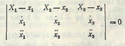
This equation represents a line passing through the point (a,) with its direction cosines proportional to b_{. Equation x_t = a, ■$- ub_t can also be written:

Xi — flt x₂ — q₃ x₃— a₃

b. ~~ b, F. •

Obligatory Words and Word Combinations

path (n), space (n), motion (n), select (n), screw (n), for short, direction cosine.

^§2 (ti

When we change the parameter on the curve from и to u_x the arc length⁶' retains its form, with и_г instead of u. We can

V5S'

8.1

•express this invariance under parameter transformations with the equation

(3) which is independent of a.

When we now introduce s as parameter instead of и — which is always possible, since ds/du <> 0 — then Eq. (3) shows us that

(4)

The vector dx/ds is therefore a unit vector, ft has a simple geometrical interpretation. The vector Ax joins two points P (x) and Q (x + Ax) on the curve. The vector Ax/As has the same direction as Ax and for As -> 0 passes into a tangent vector at P. Since its length is 1 we call the vector

(5) t = dxjds

the unit tangent vector to the curve at P. Its. sense is that of increasing s. Since

(6)

which means the limiting position of a plane passing through three nearby points of the curve when two of these points approach the third. For this purpose let us consider a plane

(7)

X generic point of the plane, a _|_ plane, p a constant, passing through the points P, Q, R on the curve given by X = x (u₀), X = x (u₁), X = x (u₂). Then the function

(8)

satisfies the conditions

and

Hence, according to Rolle's theorem, there exist the relations

and

When Q and R approach

writing u for u₀, we obtain the conditions:

we see that x = dx/du is also a tangent vector, though not ne­cessarily a unit vector.

We often express the fact that the tangent is the limiting position of a line through P and a point Q in the given inter­val of u, when Q -> Р, by saying that the tangent passes through two consecutive points on the curve. This mode of expression seems unsatisfactory, but it has considerable heuris­tic value and can still be made quite rigorous.

(9)

Eliminating a from Eqs. (9) and (7) we obtain a linea: relation between X — x, x, x (all _|_ a):

Obligatory Words and Word Combinations

invariance (n), unit vector, tangent vector, limiting (a), •mode (n), rigorous (a).

§3

The tangent can be defined as the line passing through two consecutive points of the curve. We shall now try to find the plane through three consecutive points of the curve,

arbitrary constants,

in coordinates

(10b)

Obligatory Words and Word Combinations

osculating (a), nearby (a), generic point.

67

Obligatory Words and Word Combinatlbas

§4

The line in the osculating plane at P perpendicular to the tangent line is called the principal normal. In its direction we place a unit vector n, the sense of which may be arbitrarily selected, provided it is continuous along the curve. If we now take the arc length as parameter:

(И)

where the prime signifies differentiation with respect to s then we obtain by differentiating t ■ t = 1: (12)

This shows that the vector t' = dt/ds is perpendicular to t, and since

(13)

we see that t' lies in the plane of x and x, and hence in the osculating plane. We can therefore introduce a proportionality factor k such that

(14)

The vector k = dt/ds, which expresses the rate of chant, of the tangent when we proceed along the curve, is called tl curvature vector. The factor k is called the curvature; | к is the length of the curvature vector. Although the sense of may be arbitrarily chosen, that⁷⁵'' of dt/ds is perfectly dete: mined by the curve, independent of its orientation; when changes sign, I also changes sign. When n (as is often done is taken in the sense of dt/ds, then k is always positive.

When we compare the tangent vectors t (u) at P an t + At (u + h) at Q by moving t from P to Q, then t, £ and t + At form an isosceles triangle with two sides equi to 1, enclosing the angle Aф, the angle of contingency. Sine of higher order in A<j we find for Aф -»-0:

(15)

which is the usual definition of the curvature in the case of a plane curve.

From Eq. (14) follows:

principal normal, place (v), signify (v), proportionality factor, proceed (v), curvature vector.

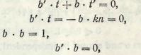
The curvature measures the rate of change of the tangent when moving along the curve. We shall now introduce a quantity measuring the rate of change of the osculating plane. For this purpose we introduce the normal at P to the osculating plane, the binormal. In it we place the unit binormal vector b in such a way that the sense t -> n -» b is the same as that⁷⁵-³ of OX -> OY -> OZ; in other words, since t, n, b are mutually perpendicular unit vectors, we define the vector b by the formula:

(17)

These three vectors t, n, b can be taken as a new frame of reference. They satisfy the relations

(18)

This frame of reference, moving along the curve forms me moving trihedron.

The rate of change of the osculating plane is expressed by the vector

This vector lies in the direction of the principal normal, since, according to the equation b ■ t = 0,

and, because

so that, introducing a proportionality factor т,

(19)

We call т the torsion of the curve. It may be positive or negative, like the curvature, but where the equation of the curve defines only k², it does" define т uniquely.

58

59

Obligatory Words and Word Combinations

binormal (n),.unit binormal vector, mutually perpendicu. 3ar, frame of reference, trihedron (n), torsion (n).

TEXT FOURTEEN

ELEMENTARY THEORY OF SURFACES

§1

We shall give a surface, in most cases, by expressing its rectangular cporjiiriates x_t as functions of two parameters

u, v in a certain closed interval:

(1)

The conditions imposed on these functions, are analogous to those⁷⁵'* imposed on the conditions for curves. We consider the functions x_t to be"⁹ real functions of the real variable;: u, v, unless imaginaries are explicitly introduced. When the functions are differentiable to the order n — 1, and the n-th derivatives exit, we can establish the Taylor formula:

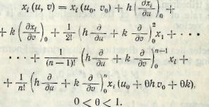
When we write the equation of the surface in vector form:

quation of the surface in vector form:

(4)

(4)

the condition that the rank of matrix M be can be written jn the form

the condition that the rank of matrix M be can be written in the form

(5)

.

This equation allows a simple geometrical interpretation. When we keep i constant in Eq. (1) or Eq. (4), the x depends on only one parameter и and thus determines f curve on the surface, S parametric curve, v = constant. Similarly, и = = constant represents another parametric curve. When the constants vary, the surface is covered with a net of parametric curves, two of which pass through every point P, forming the family of oo curves v=constant and the family of oо¹ curves lu = constant At P the vector x_u is tangent to the curve v = = constant, and x_v is tangent to the curve и = constant. Condition (5) means that at P the vectors x_u and x„ do not vanish and have different directions.

We also call (u, v) the curvilinear coordinates of a point 'on the surface. As curvilinear coordinates of a point on the sphere we may select latitude and longitude, a familiar pro­cedure in geography; polar coordinates are an example of curvilinear coordinates in the plane (rectilinear coordinates) can be considered as a special case of curvilinear coordinates). The parametric curves are also called coordinate curves.

Obligatory Words and Word Combinations

representation (n), explicitly (adv), differentiable (a), rank of matrix, allow (v), parametric curve, net of curves, curvili­near coordinates, latitude (n), longitude (n), polar coordinates, rectilinear coordinate curves.

has rank 2.

The parameters и and v must be independent, which means that the matrix

§2

A relation ф (u, v) = 0 between the curvilinear coordinates determines a curve on the surface. Such a curve can also be given in parametric form:

(6) u = u(0, v = v(t).

61

The vector dx/dt = x, at a point P of the surface, given by

(7) x = x_uu+ x_vv

is tangent to the curve and therefore to the surface. Eq. (7) can be written in a form independent of the choice of parame­ter:

(8) dx = x_udu + x„dv.

When the curve is given by 9 (и, v,) = 0, the du and da are connected by the relation

(9) ф_udu + ф_vdv = 0.

The ratio dv/du = —ф_u/ф„ is sufficient to determine the direc­tion of the tangent to the surface.

The distance of two points P and Q on a curve is found by integrating

(10)

along the curve; and substituting for dx the values (7), we find

where

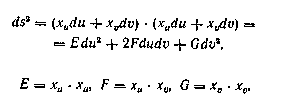
The E, F, G are functions of и and v. The distance between P and Q on the curve и — и (t),v = v (t) can now be expressed as follows:

The expression (11) for ds is called the first fundamental form of the surface. It is a quadratic differential form; its square root ds can be taken as the length [ dx | of the vector differential dx on the surface, and is called the element of arc. Since ds is a length,

is always positive (except zero for du = dv = 0), as long as ^ss we study real surfaces; such a form is called positive definite.

is always positive (except zero for du = dv = 0), as long as ^m we study real surfaces; such a form is called positive definite.

With the aid of E, F, G we can express the angle a of two tangent directions to the surface given by du/dv, 6u/Sv. Then

dx = x_udu + x_vdv, 6x = x_u8u + x_v6v and

The following cases of Eq. (13) are particularly important:

1. When a = л/2 we obtain the condition of orthogonality of two directions on the surface:

I (14)

2. The angle 0 of the parametric lines и — constant (hence du = 0, dv arbitrary) and v = constant (hence 6u arbitrary, ov — 0), is given by

(15)

3. The parametric curves are orthogonal if F — 0.

Obligatory Words and Word Combinations

connect (v), integrate (v), first fundamental form of the surface, quadratic differential form, square root, element of arc, aid (n), orthogonality (n).

§3

All vectors dx/dt through P tangent to the surface satisfy the Eq. (7) and therefore lie in the plane of the vectors x_a and x„ uniquely determined at all points where х_и *х_а <>0 (compare with Eq. (5)). This plane is the tangent plane at P to the surface. Its equation is

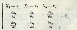
(16a) X = x + Xx_u + u,x„, X, u parameters or

(16b)

where the derivatives are taken at P (x_v x_%, x₃).

₆₃

The surface normal, normal for short"³, is the line at P perpendicular to the tangent plane. As unit vector in this normal we take:

(17)

We also might have taken * — N as unit normal vector, since the sense of N depends on the labelling of the coordinate curves. Since

(18)

we conclude from Eq. (2), using the theory of contact:

The tangent plane has, of all planes through P, the highest

contact with the surface. This contact is of order one.

In the books on the calculus it is shown that the area of

a region R on the surface is given by

The formula can be made plausible by the consideration that the area of a small parallelogram bounded by the two vectors dx and bx is

— 6udu\.Taking for dx and их vectors tangent to the coordi­nate lines (6u = 0, du — 0), and writing du for &v (in accor­dance with the established custom of integration theory), we obtain

(19)

(19)

Obligatory Words and Word Combinations

normal (n), unit normal vector, label (v), conclude (v), tan­gent plane, contact (n), region (n), plausible (a), coordinate line, in accordance with.

§4

Tangent developables share with cones and cylinders the property that they have a constant tangent plane along a gene­rating line. Their tangent planes therefore depend on only one parameter. Such surfaces can be considered as the envelope of a one-parameter family of planes. We shall show that they are

64

the only surfaces that can be considered as the envelope of such a family of oo planes.

Such a family can be given by the equation

(20)

where the a and p depend on a parameter u. We exclude the case that

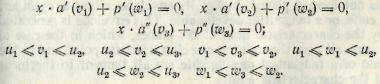
which gives a family of parallel planes, as does²⁰ the case that a and a' are collinear. The planes determined by the parameters и = u₁ and и = и₂ (u₁ < u₂) then intersect in a straight line, which also lies in the plane

or, according to the mean value theorem,

When u_2-»u₁ we find that this line takes a limiting posi­tion given bv

(21)

This line is called me charactenstic 0f the plane.

The planes determined by the parameters и = u_lt и = u₂, and a = u₃ {u_l < w₂ < u_s) intersect in a point, which also lies in the planes

When u₃ -> u₂ -> и_г we find that this point takes a li­miting position given bv (22)

This point is called the characteristic point of the plane (20). It lies on the characteristic line. It does not exist when (aa'a") = 0,in which case the vector field a (u) is plane. But the vector a is perpendicular to plane (20). When the vectors a (u) are parallel to a plane it, the planes (20) are all parallel to the direction perpendicular to n. In this case the envelope of the planes (20) is therefore a cylinder with generating lines perpendicular to the plane u (except in the case that the planes form a pencil and the «envelope» is a straight line).

; 65

When the characteristic point is the same for all planes the envelope is a cone generated by all characteristic lines.

In the general case there exists a locus of characteristic points, which is a curve C. We shall show that the characte­ristic line is tangent to С at its characteristic point. For this purpose let us consider Eq. (22) solved for x, which then becomes a function of u. Differentiation of the first two equa­tions of (22) shows that

whicn, when compared with tq. (zz), gives

(23)

This means that the tangent vector x' to С has the direction of line (21). Since it passes through the characteristic point, x' must lie in the characteristic line. Similarly, differentiating the first equation of (23), we obtain

Comparing this with the second equation of (23) we find that x" ■ a = 0, which with x' ■ a = 0 means that the vector x'*x" is parallel to a. The osculating plane of the curve С at the characteristic point is therefore identical with the plane (20). We have thus found the following theorem.

A family of oo¹ planes, which are not all parallel and which do not form a pencil, has as its envelope either a cylinder, a cone, or a tangential developable. This envelope is generated by the characteristic lines of the planes, which in the case of a cone all pass through the one characteristic point and in the case of a tangential developable are all tangent to the locus of the characteristic points.

The locus of the characteristic points is called the edge of regression. It reduces to a point in the case of a cone. Its name is due to⁸³ the fact that the intersection of a tangen­tial developable with the normal plane to this edge of regression at one of its points P has a cusp at that point.

Obligatory Words and Word Combinations

developable surface, cone (n), cylinder (n), generating line, envelope of a family of planes, parallel planes, collinear pla­nes, intersect (v), mean value theorem, characteristic point (line), vector field, pencil (n), tangential (a), edge of regression, cusp (n).

§5

The geometry of surfaces depends on two quadratic diffe­rential forms. We have already introduced the first of them, which represents ds². The second fundamental form can be obtained by taking on the surface a curve С passing through a point P, and considering the curvature vector of С at P. When t is the unit tangent vector of C, this curvature vector k is equal to dt/ds. We now decompose k into a component k_a normal and a component k_g tangential to the surface:

(24) dt/ds = к = к„ + к_г.

The vector k_n is called the normal curvature vector and can be expressed in terms of the unit surface normal vector N:

(25) k_n = k„N,

where k is the normal curvature. The vector k_n is determined by С alone (not by any choice of the sense of t or N), the scalar k, depends for its sign on the sense of N. The vector kg is called the tangential curvature vector or geodesic curva­ture vector. We shall deal in this section with the properties of k„.

From the equation N • t = 0 we obtain by differentiation along C:

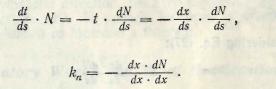
(26)

or

(27)

Let us study first the right-hand side of this equation.

Both N and x are surface functions of и and v (which

in their turn depend on C). With the aid of resulting identities

(28)

we can write Eq. (27) in the form:

66

In this equation

.30)

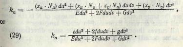
are functions of и and v, which depend on the second deri­vatives of the x with respect to и and v, in this respect diffe­ring from E, F, G, which depend on first derivatives only. We write the denominator and numerator of Eq. (29) in the following form:

I is the first fundamental form, II the second fundamenta form. Since x_u ■ N — 0 and x_v ■ N = 0, we can also write fo e, f and g:

Obligatory Words and Word Combinations

second Fundamental form, normal curvature vector, unit surface normal vector, scalar (n), tangential (geodesic) curva­ture vector.

§6

or, what is its equivalent, Eq. (29):

Considering Eq. (27):

we see that the right-hand side depends only on u, v, and dv/du. The coefficients e, f, g, E, F, G are constants at P, so that k_n is fully determined, at P, by the direction dv/du. All curves through P tangent to the same direction have the­refore the same normal curvature (if the sense of N is the same for all these curves). Expressed in vector language:

All curves through P tangent to the same direction have the same normal curvature vector.

68

When we momentarily give to N the sense of k_n, and to n the sense of dt/ds, then we can express this theorem in the form obtained from Eq. (26):

When we momentarily give to N the sense of k_n, and to n the sense of dt/ds, then we can express this theorem in the form obtained from Eq. (26):

( 33)

is the angle between N and n.

where ф (0 < <ф < pi/2) is the angle between N and n. This equation can be expressed in another form for directions t for which k_n <>0, hence also k <> 0. Such directions are called nonasymptotic directions. For curves in such directions we can write P = k^-1, R_n = k^-1. The quantities P and P„ are here positive, P represents the radius of curvature of a curve with tangent t and cp = 0. One such curve is the intersection of the surface with the plane at P through t and the surface normal; this curve is called the normal section of the surface at P in the direction of С Eq. (33) now takes the form

(34)

We can thus express our previous theorem in the following form:

The center of curvature C_x of a curve С in a nonasymptotic direction at P is the projection on the principal normal of the center of curvature C₀ of the normal section which is tangent to С at P. And in still other words:

If a set of planes be drawn through a tangent to a surface in a nonasymptotic direction, then the osculating circles of the intersections with the surface lie upon a sphere. This theorem is known as Meusnier's theorem.

Obligatory Words and Word Combinations

§ 7

The normal curvature in direction du/dv is given by Eqs. (29):

. _ edu* + 2fdudv+gdv* __ e + 2/X + gl' _ , .. Edu? + 2Fdudv + Qdifl ~ E + 2F1 + OX' ~ ^W' (35)

where Л = dv/du. The extreme values of k can be characterized by dk/dl = 0:

where X. = dv/du. The extreme values of k can be characterized by dk/dl = 0:

(E + 2F + G^a)(/ + g)-(e + 2/ + g*)(F + G) = 0.

69

Since

we can, in this case, express Eq. (35) in a simpler form:

Elimination of k gives a quadratic equation for

(36) Hence k satisfies the equations

or

= 0.

(37b)

This equation determines two directions dv/du, in which k obtains an extreme value, unless II vanishes or unless II and I are proportional. One value must be a maximum, the other a minimum. These directions are called the directions of principal curvature, or curvature directions. They are determined either by Eqs. (36a), (37a), or (37b). Since the roots л_v л_г satisfy the equation (compare with Eq. (37a)):

the curvature directions are orthogonal (according to E,q. 14). This also holds for the case that gF — Of — 0, when, accord­ing to Eq. (37b), one of the directions is dus= 0. We call the normal curvatures in the curvature directions the principal curvatures, and denote them by k_x and k₂-

Integration of Eq. (37) gives us the lines of curvature on the surface, which form two sets of curves intersecting at right angles, or an orthogonal family of curves on the surface. From the existence theorem of ordinary differential equations, we can conclude that these curves cover the surface simply and without gaps in the neighbourhood of every point where the coefficients of the first and second fundamental forms are

70

continuous, except at the points where these coefficients are proportional. Such points are called navel points or umbilics, and we exclude them for the moment. Now let us take the lines of curvature as the parametric lines. Then Eqs. (37a, b) must be satisfied for du = 0, dv arbitrary, and for dv = =0. du arbitrary. Hence:

In these equations F = 0 because the parametric lines are orthogonal; moreover, neither E nor G can be zero (EG — F² > > 0). We therefore find that when the parametric lines are lines of curvature:

(38) F = 0, f = 0.

This condition is necessary, and, because of Eq. (37b), also sufficient. Now Eq. (35) takes the form:

(39)

This formula can be expressed in a simple form. We find by substituting first dv = 0, then du — 0, into Eq. (39), that

(40)

and if we introduce the angle a between the direction dvjdu and the curvature direction 6v = 0, we find from Eq. (14)

that

(41) Eq. (39) therefore takes the form:

(42)

This relation, which expresses the normal curvature in an arbitrary direction in terms of k_x, k,, is known as Euler's theorem. Together with Meusnier's formula it gives full in­formation concerning the curvature of any curve through P on the surface.

Obligatory Words and Word Combinations

elimination (n), curvature direction, principal curvature, existence theorem, differential equation, gap (n), navel

Point iimhili>

71

TEXT FIFTEEN

SOME CONCEPTS OF AFFINE GEOMETRY AND PROJECTIVE GEOMETRY

< ,-^//л/^-V -'j -

. The ordinary geometry taught in school, dealing with circles, angles, parallel lines, similar triangles and so on, is called Euclidean geometry because it was first collected into a systematic account by the Greek geometer Euclid, who lived about 300 В. С His tfe'atise', the Elements, is one of the most famous^boplis, in the world.

During the nineteenth century there was a tendency to extract from Euclidean.geometry certain ideas'of a particularly simple naliire, Especially lMea's that did not involve measure­ment of a distance or angle, and to use these for building up more general systems, notably affine geometryand projective geometry.

These two systems are said to beⁿ more general because, besides throwing''* fresh light on Euclidean geometry itself, they are capable of extension in other directions by the intro­duction of new kinds of measurement. Affine geometry can be developed into Minkowski's geometry of the space-time conti­nuum considered in the special theory of relativity, and pro­jective geometry can be developed into the various kinds of 'non-Euclidean' geometry that are relevant to more modem ideas of relativistic cosmology.

Obligatory Words and Word Combinations

affine geometry, projective geometry, collect (v),-account (n), extract (v), measurement (n), space-time continuum, relevant (a).

§2

Two figures in distinct planes are said to be derived¹¹ from each other by parallel projection if corresponding-points can be joined by parallel lines. If the two planes are parallel, the two figures will be exactly alike (congruent); otherwise they may have somewhat different slopes, but straight lines remain straight, tangents to curves remain tangent, parallel

72

lines remain parallel, bisected segments remain bisected, and equal areas remain equal. In other words, the properties of straightness, tangency, parallelism, bisection and equality ₀f area are invariant under parallel projection. Such properties are the subject-matter of affine geometry. (The use of the word 'affine' is due to⁸³ the Swiss mathematician Euler, 1707—83).

On the otiier hand*³, the content of projective geometry is still more restricted, being confined to those properties (such as straightness and tangency) which remain invariant under central projection.

Two figures in distinct planes are said to be derived from each other by centra! projection if corresponding points can be joined by concurrent lines, all passing through a fixed point L. If the two planes are parallel, the two figures will be similar and the invariant geometry will again be affine.

The study of projective properties of figures which remain unchanged under central projection lay the foundation of a new branch of geometry, synthetic projective geometry. The new geometry was constructed by a remarkable Frenchman, Jean Victor Poncelet (1788—1867).

Obligatory Words and Word Combinations

parallel projection, alike (a), content (n), central projec­tion, concurrent lines, lay the foundation, remarkable (a).

§ 3

We defined affine geometry as consisting of those proposi­tions of Euclidean geometry which retain their meaning and validity after parallel projection; thus every proposition of affine geometry holds also in Euclidean geometry, but other propositions of Euclidean geometry are essentially meaningless in affine geometry. Somewhat similarly, projective geometry includes all propositions of affine geometry that retain their meaning and validity after central projection; but this is not the whole story. Some statements are true in projective geo­metry but false in affine geometry. The most important in­stance is: 'Any two lines in a plane have a point of intersec­tion'. This fails in affine geometry because the two lines might be parallel. The projective statement is validated by inventing a new kind of 'point' so as to be able to say that parallel lines

73

have a common point at infinity: the projected image of a point on the vanishing line. This vitally important concept is due to the great German astronomer Kepler (1571—1630). We often think of'a line as consisting af all the points on it, i. e. a range of points. It is equally useful to think of a point as consisting of all the lines through it, i. е. a pencil of lines. Statements about points are easily translated into statements about pencils; e. g. 'Two points lie on just one line' becomes 'Two pencils contain just one common line'.- Lines through a point A project into parallel lines on the horizontal plane. If we agree to call these a pencil of paral­lels, we may say that a pencil always proj.ects into a pencil. When statements about such pencils are translated back into statements about points, we have to admit points at infinity as well as ordinary points. In fact, we call the pencil of paral­lels a point at infinity.

Obligatory Words and Word Combinations

validity (n), essentially (adv), fail (v), invent (v), range (n), pencil of parallels, admit (v), point at infinity.

§4

We have extended the meaning of the word 'point' so as to be able to say that any two coplanar lines intersect in a point. Similarly, we extend the meaning of the word 'line' so as to be able to say that any two planes intersect in a line. If the two planes happen to be parallel, this is a line at infinity.

For a complete treatment of "ideal elements" we should'" have¹' to consider the whole space, using bundles of lines and planes (i. e. all the lines and planes through a given poini or parallel to a given line) instead of pencils of lines. Then a 'point' is said to lie⁷¹ in a plane if the plane belongs to the bundle; and in the case of a bundle of parallels this merely means that the plane contains a line in the direction of the bundle. When we restrict consideration to a single plane, the bundle is replaced by a pencil, all the lines of an ordinary pencil contain different points at infinity (which belong equal­ly to the respectively parallel lines of any other ordinary pen­cil), and all these points at infinity ате^ш to be regarded as a range on the line at infinity. We can treat the points at in­finity just like any other range of points so long as we are

74

dealing with properties that are invariant under central pro­jection.

We have enlarged the affine plane (in which both the affine and Euclidean geometries operate) so as to obtain the projective plane, which has simpler properties of incidence.

Obligatory Words and Word Combinations

coplanar (a), bundle of planes (lines), belong (v), single (a), equally (adv), treat (v), enlarge (v), incidence (n).

TEXT SIXTEEN PROBABILITY THEORY

§1

We often hear statements of the following kind: "It is likely to rain today", "I have a fair chance of passing this course", "There is an even chance that a coin will come up heads", etc. In each case our statement refers to a situation in which we are not certain of the outcome, but we express some degree of confidence that our prediction will be verified. The theory of probability, provides a mathematical framework for such assertions.

Consider an experiment whose outcome is not known. Suppose that someone makes an assertion p about the outcome of the experiment, and we want to assign a probability to p. When statement p is considered in isolation, we usually find no natural assignment of probabilities. Rather, we look for a method of assigning probabilities to all conceivable state­ments concerning the outcome of the experiment. At first this might seem to be a hopeless task, since there is no end to the statements we can make about the experiment. However we are aided by a basic principle:

Fundamental assumption: Any two equivalent statements will be assigned the same probability.

As tongas⁸⁵there are a finite number of logical probabilities, there are only a finite number of truth sets?², and hence the pro­cess of assigning probabilities is a finite one. We proceed in three steps: (1) we first determine U, the aossibtlity set"¹, that

is, the set of all logical possibilities, (2) to each subset X of (j we assign a number called the measure m (X), (3) to each statement p we assign m (P), the measure of its truth sets, as a probability. The probability of statement p is denoted by Pr [p].

It is important to remember that there is no unique method for analyzing logical possibilities. In a given problem we may arrive at a very fine or a very tough analysis of possibilities, causing U to have many or few elements.

Having chosen U, the next step is to assign a number to each subset X of U, which will in turn³³ be taken to be the probability of any statement having truth set X.

Obligatory Words and Word Combinations

probability theory, it is likely, situation (n), certain (a), outcome (n), degree (n), prediction (n), however (adv), as long as, truth set, possibility set, measure (n), in* turn.

§2

Assign a positive number (weight) to each element of (J, so that the sum of the weights assigned" is 1. Then the measure of a set is the sum of the weights of its elements. The measure of the set e is 0.

In applications of probability theory to scientific problems, the assignment of measures and the analysis of the logical possibilities may depend upon factual information and hence can best be done^by the scientists making the application. И*'-' Once"¹-⁶ the weights are assigned, to find the probability of a particular statement we must find its truth set and find the sum of the weights assigned to elements of the truth set. This problem, which might seem easy, can often involve conside­rable mathematical difficulty. The development of techniques^8S to solve this kind of problem is the main task of probability theory.

Example. An ordinary die is thrown. What is the probabi­lity that the number which turns up is less than 4? Here the probability set is U = (1,2, 3, 4, 5, 6). The symmetry of the die suggests that each face should have the same probability

of turning up ²⁵. To make this so we assign weight -g- to each

of the outcomes. The truth set of the statement, "The number

_which turns up is less than 4" is(l, 2, 3). Hence the probabili­ty of this statement is -|- = -g-, the sum of the weights of the elements in its truth set.

Obligatory Words and Word Combinations

weight (n), scientific (a), scientist (n), assignment (n), infor­mation (n), once (cj) considerable (a), technique (n), symmet­ry (n), suggest (v), face (n), turn up (v).

I § ³

We shall consider some general properties of probability measures which are useful in computations and in the general understanding of probability theory.

Three basic properties of a probability measure" are:

1. m (X) = 0 if and only if X = e.

2. 0 < m (X) < 1 for any set X.

(Q For two sets X and Y, m (XUY) = m (X) + m (Y) if and only if X and Y are disjoint, i. e. have no elements in common^8S.

We shall prove (C).

We observe first that m (X) + m (Y) is the sum of the weights of the elements of X added to the sum of the weights of Y. If X and Y are disjoint, then the weight of every element of XUY is added once and only once, and hence m (X) + + m(Y) = m(xUY).

Assume now that X and Y are not disjoint. Here the weight of every element contained in both X and Y, i.e. in Xf]Y, is added twice in the sum m (X) + m (Y). Thus this sum is greater than m (XUY) by an amount m (X [) Y). By (A) and (B), if Xf] Y is not the empty set, then m(X(\Y) > 0. Hence in this case we have m (X) + m (У) > т (XUY). Thus if X and Y are not disjoint, the equality in (C) does not hold. Our proof shows that in general we have

(C) For any two sets X and Y,

m(XUY) = m(X) + m(Y)-m(X()Y).

Since the probabilities for statements are obtained directly from the probability measure m (X), any property of m (X) can be translated into a property about the probability of statements. For example, the above properties become, when expressed" in terms of statements:

76

77

1. Pr [p] = 0 if and only if p is logically false.

2. 0 < Pr [p]< 1 for any statement p.

3. The equality

Pr\pVq] = Pr[p] + Pr[q]

holds if and only if p and q are inconsistent, (c') For any two statements p and q,

Pr [pVq] = Pr [p] + Pr [q] — Pr [p/\q\.

Another property of a probability measure which is often useful in computation is

(D) m(X) = \ — m(X),

or, in the language of statements,

(d) Pr[~~p\ = \-Pr\p\.

Obligatory Words and Word Combinations

computation (n), disjoint (a), in common, twice (adv), emp­ty (a), translate (v), above (a), false (a), inconsistent (a).

1/ §4

There are occasions in probability theory when one finds a problem for which the answer, based on probability theory, is not at all*³ in agreement⁸³ with one's intuition. A particularly good example of this is provided by the matching birthdays problem.

Assume that we have a room with r people in it and we pro­pose the bet that there are at least⁸³ two people in the room having the same birthday, i. e. the same month and day of the year. We ask for the value of r which will make this a fair bet. Few people would be willing to bet even money unless there were³³ at least 100 people in the room. Most people would³ suggest 150 as a reasonable number. However, we shall see that with 150 people the odds are approximately 4,500,000,000,000,000 to 1 in favour of two people having the same birthday, and that one should*¹ be willing to bet even money with as few as 23 people in the room.

Let us first find the probability that in a room with r people, no two have the same birthday. There are 365 possibi­lities for each person's birthday (neglecting February 29). There are then 365^л possibilities for the birthdays of r people.

78

We assume that all these possibilities are equally likely. To find the probability that no two persons have the same birth­day we must find the number of possibilites for the birthdays

i which have no day represented twice. The first person can have any of 365 days for his birthday. For each of these, if the second

I person is to have a different birthday, there are only 364 possibilities for his birthday. For the third man, there are 363 possibilities, if he is to have a different birthday than the first two, etc. Thus the probability that no two people have the same birthday in a group of r people is

f_ 365 -364 (365— r+ 1) г = 23 P, = 0,507.

Obligatory Words and Word Combinations

occasion (n), not at all, in agreement with, value (n), un­less (cj), reasonable (a), approximately (adv), in favour of, as few as.

§5

Suppose³" that we have a given set U and that measures have been assigned to all subsets of U. A statement p will have probability Pr [p] = m (P). Suppose we now receive some additional information, say³' that statement q is true. How does this additional information alter the probability of p?

The probability of p after the receipt of the information

q is called its conditional probability, and it is denoted by

Pr [p\q], which is read "the probability of p given?". In this

' section we will construct a method of finding this conditional

probability in terms of the measure m.

If we know that q is true, then the original possibility set £/ has been reduced to Q and therefore we must define our measure on the subsets of Q instead of on the subsets of U. Of course, every non-empty subset X of Q is a subset of U, and hence we know m (X), its measure before q was discovered. Since q cuts down on the number of possibilities, its new measure m' (X) should be large.

The basic idea on which the definition of m' is based is that, while we know that the possibility set has been reduced

79

to Q, we have no new information about subsets of Q. If X and Y are subsets of Q, and m (X) = 1 ■ m (Y), then we wilV want m' (X) = 2 ■ m' (У). This will be the case*² if the measures of subsets of Q are simply increased by a propor­tionality factor** m' (X) = k ■ m (X) and all that remains is to determine k. Since we know that i = m' (Q) = k ■ m (Q), we see that k = 1/m (Q), and our new measure on subsets of U is determined by the formula

^v ' m (Q) How does this affect the probability of p? First of all the truth set of p has been reduced. Because all elements of Q have been eliminated, the new truth set of p is P(]Q and therefore

(2) _P,_[pl„ _{= m4PnQ) =} ^™ ₌ ^ML.

Example. At a chess tournament for world 'championship challenger A has 0.4 chance of winning, В has 0.3 chance, С has 0.2 chance, and D has 0.1 chance. Just before the tourna­ment С withdraws. What are now the chances of the other three challengers? Let q be the statement that С will not win, i. e. that A or В or D will win. Observe that Pr [q] = 0.8, hence all the other probabilities are increased by a factor of 1/0.8 = 1.25. Challenger A now has 0.5 chance of winning, В has 0.375, and D has 0.125.

Obligatory Words and Word Combinations

additional (a), receipt (n), conditional probability, cut down (v), proportionality factor, affect (v), first of all, eli­minate (v).

TEXT SEVENTEEN TOPOLOGICAL SPACE

§ 1

A topological space is a set X in which certain subsets, called open sets, are distinguished; the collection of open sets satisfies the axioms:

1. the union of any number of open sets is open;

1. the intersection of any finite number of open sets is open;

2. the whole space and the empty set are open.

To prescribe the open sets is to assign a topology to the set X. If V, V are two topologies on the set X, then U is finer than V (V is coarser than U) if every set of X which is open in the topology V is open in the topology U. A set of open sets of X forms a base (for the open sets) if every open set $ X is a union of sets of the base.

i A closed subset of the topological space X is the comple­ment of an open set; thus a topology is assigned by prescribing the closed sets and the closed sets must satisfy the axioms:

CI the union of any finite number of closed sets is closed;

C2 the intersection of any number of closed sets is closed;

C3 the whole space and the empty set are closed.

If X₀ is a subset of the topological space X, the induced topology in X₀ is that in which the open sets are the inter­sections with X₀ of the open sets of X. Subsets will always be supposed to carry''¹ the induced topology. Plainly, if Xj s X, С X, then X„ and X induce the same topology in X_v and an open (closed) subset of an open (closed) subset of X is an open (closed) subset of X.

The interior of X₀ is the union of all open subsets of X contained in X₀. The interior of X„ is the largest open set contained in X₀.

The closure of X₀ is the intersection of all closed sets con­taining X₀. The closure of X₀ is the smallest closed set con­taining X₀.

If x £ X, a neighbourhood of x in X is a subset of X con­taining x in its interior. The closure of X₀ is the sets of points x £ X such that every neighbourhood of x meets X₀.

The frontier of X₀ in X is the intersection of the closure of X₀ and the closure of its complement. X₀ is dense in X if

its closure is X. The sequence x_v x₂ x_n, ... of points of X

converges to x £ X if every neighbourhood of x contains all but a finite number of points of the sequence.

The collection (X,) of subsets of X is a covering of X if their union is X. The covering is open (closed) if each j|j is open (closed). The covering is finite (countable) if there are finitely many (countably many) sets in the covering. The covering (Ky) is a subcovering (refinement) of the covering l*i) if each Y/ is (is contained in) an X,-.

81

Obligatory Words and Word Combinations

topology (n), topological space, open (closed) set, union (n), fine (a), coarse (a), base (n), complement (n), induced (a), plainly (adv), closure (n), frontier (n), covering (n), count­able (a), refinement (n).

§2

A map /: X -► Y from the space X to the space К is a continuous function from X to Y; the continuity of / is expres­sed by the property that, if U is any open subset of Y then f"¹ (U), the set of points of X mapped by / into U, is open in X. Equivalently, / is continuous provided f~' (F) is closed whenever F is closed. If X_e sg X, then X₀/ is the set of points xf, x £ X₀, and is called the /-image of X₀. If У„ с Y, f¹ (Y₀) is called the /-counterfmage of Y₀. A map f: X -»■ Y determines functions /₀: X₀ -> Y, /' : X -* Xf given by ^xfa — ^xf> ' 6 -f il xf = xf, x £ X. We nfay write /₀ as f\X₀, and we say that/₀ is the restriction of / to X₀ and that / is an extension of /₀ to X, or over X. The functions /„, f are continuous.

Let \A_t) be a finite covering of X by closed sets and let f_t:A_t-+Y be maps such that f,\A, (] A/ = f/\A, f] A/. Then we may define a unique function: f: X -* Y by f j A_t = f_t. The function f: X -*- Y is continuous. (For if F g; У is closed then r^lF =f(J.,fT' (F); but />.' (F) is closed in Д, and hence in X so that, by (CI), f~'F is closed in X and / is continuous). A similar result holds for arbitrary coverings by open sets.

If X₀ s X, let i : X₀ -y X be given by xi = x, x £ X₀. Then i is plainly continuous and we call it an inclusion map or injection. If there exists a map p : X -* X₀ such that ip = 1, where 1 is the identity map of X₀, then X₀ is a retract of X and p is a retraction.

The map / : X ->- Y is a homeomorphism of X onto К (abbreviated to homeomorphism) if there is a map g : К -*- X (called the inverse of /) such that fg = 1 : X ->- X and gf = = 1 : У — У. We write / : X ss У and say that X and У are homeomorphic or of the same topological type. X s У is an equivalence relation.

The map / : X -> У is a homeomorphism of X into У if the induced map f : X -* X/ is a homeomorphism. Plainly (': X„ is a homeomorphism of X„ into X; if / : X ->- У is a

82

homeomorphism of X into У, then X may be embedded in Y by identifying x with xf, x £ X. The map / : X ->- У is locally (lomeomorphic if each x £ X possesses a neighbourhood V such that f maps U homeomorphically onto a neighbourhood

(f xf. Let / : X -*- У be a function from the space X onto the :t У; then the identification topology on У determined by / is the topology in which У₀ s У is closed if and only if K~' (У₀) is closed. If У is given the identification topology, | is called an identification map or projection. The identi­fication topology is the finest topology consistent with the continuity of /.

Let R be an equivalence relation on the points of X (thus xRx; xRx' implies x'Rx; xRx' and x'Rx" together imply xRx". Let У be the set of /^-equivalence classes and let k : X ->■ -> У send each point to its equivalence class. If У is given the identification topology determined by k we may write Y = X \R and say that У is the quotient space of X by the relation R (with the quotient topology).

Given two spaces X and У their topological product X X У ;is the set of pairs (x, y), x £ X, у £ Y, with the topology in which a base of open sets consists of the sets U X У, where U is open in X and У is open in У. The maps (x, y) -> x, {x, y) -*y project X X У onto X, У. If x, £ X, y, £ Y, the maps x ->- (x, {/„.), у ->- (x_t, y) embed X, У in X X У; we refer to these maps as injections.

The subspace (X X y„) U (x_t X У) of X X У is called the bunch of X and У and is written X V У if there is no peed to specify the points x_t, y_r Then X x {/», x, X У are subspaces of X V У whose union is X V У and whose in­tersection is the single point (x^., y^). Thus, using the injections defined above, we may think of X V У as the 'union of X Bnd У with a single common point'.

Clearly the notion of topological product extends to finite collections of spaces (it also extends to infinite collections, but we shall only be concerned with finite products).

Obligatory Words and Word Combinations

map(n), (v), counterimage (n), extension (n), inclusion (n), Injection (n), retract (n), retraction (n), homeomorphism (n), homeomorphic (a), embed (v), identification topology, iden­tification map, consistent (a), quotient space, quotient topo­logy, bunch (n), specify (v), topological product.

83

§ з

A metric in the set X is a real-valued function p defined on (ordered) pairs of points of X and satisfying:

1. for x, у £ X, p (*, y) > 0;

2. p (x, y) = p (i/, x);

3. p (дг, у) = 0 if and only И x = y;

4. (triangle inequality) for x, у, г £ X, p (x, {/) + p (#,?) > > P (x, 2).

The e-ball, centre x, in the set X (with the metric p) is the set, V (x, e), of points;/ £ X withp (x, y) < e. The metric topology in the set X is the topology in which the open sets are unions of sets of the form V (дг, е). The metric topology is a topology.

X is a metric space if its topology is given by a metric p. The diameter of a subset X„ of a metric space X is sup p (x, y) x,y£X₀

The topological space X is metrizable if ttie set X admits a metric such that the metric topology coincides with the given topology. A function / : X ->- Y from the metric space X to the metric space Y is continuous if and only if, for any x £ X and e > 0, there exists 6 (x, e) = 6 > 0 such that V (x, 8) / ct V (xf, e).

The map / is uniformly continuous if 6 may be chosen in­dependently of x.

The space X is:

Hausdorff if any two distinct points of X possess disjoint neighbourhoods;

compact if every open covering of X has a finite subcove-ring;

sequentially compact if every sequence of points of X has a convergent subsequence;

locally compact if every point of X has a compact neigh­bourhood;

connected if X is not the union of two disjoint non-empty closed sets;

separable if X possesses a countable dense subset.

A metric space is compact if and only if it is sequentially compact. A compact metric space is separable. A (continuous) map of a compact metric space into a metric space is uniformly continuous. The limit of a convergent sequence in a Hausdorff space is unique. A compact subset of a Hausdorff space is closed. If X is locally compact and Hausdorff then every neigh-

bourhood contains a compact neighbourhood. A subset of Euclidean space fC is compact if and only if it is closed and bounded.

Obligatory Words and Word Combinations

metric (n), real-valued function, ball (n), metric topology, diameter (n), metrizable (a), uniformly (adv), compact (a), connected (a), sequentially (adv), locally (adv).

§4

A partially ordered set is a set A of elements and an order relation (to be read as «less than or equal to») a, < a₂ that holds between certain pairs of elements of A. This relation satisfies the conditions:

1. for all a£A,a<a\

2. if a₁ < а_г, a₂ < a₃, then a₁ < o₃.

We remark that we do not in general demand

3) if a₁ < a₂, o₂ < a_v then a_t = а_г.

A totally ordered set is a strictly partially ordered set A such that for each pair a, a' £ A either a < a' or a' < a.

Examples: (a) the real numbers, ordered by <, form a totally ordered set;

(P) the complex numbers, ordered by the relation a + ib < < a' + ib' if and only if a < a' and b < b', form a partially ordered set;

(y) the set of subsets of a given set, ordered by s, form a partially ordered set;

(6) the set of coverings of a space (or, indeed, set) X ordered by the relation |X,( < (У,) if and only if [Y,] is a refi­nement of (X,) is a partially ordered set.

Note that if (X,] is the set of all 2~"-balls in a metric space X and {Y,} is the set of all 3""-bails, n = 0, 1,2, ..., then |X,] < [Y,\ and [Y,\ < (X,) but (X,j ф \Y,\ in general.

The element b of the partially ordered set A is an upper bound of the subset 4,eJ if o₀ < b for all a₀ £ A„. A is inductive if each totally ordered subset of A has an upper bound in A. The element m £ A is maximal if for all a £ A, m < a implies a < m.

(Zorn's lemma). If the (non-empty) partially ordered set A is inductive, then it possesses a maximal element.

84

8&

If A„ is a totally ordered subset of the inductive set A, then it possesses a maximal upper bound.

(For the set of upper bounds of A₀ is inductive if A is

inductive).

Obligatory Words and Word Combinations

partially (totally) ordered set, order relation, inductive (a), maximal (a).

TEXT EIGHTEEN

PLATEAU'S PROBLEM

§ ⁷

Plateau's problem is intimately connected with Dirichlet's Principle and conformal mapping. It has long challenged ma­thematicians by the contrast between its simplicity of state­ment and difficulty of solution: to find the surface G of least area spanned in a given closed Jordan curve y. if the surface О is represented in x, y, z-space by a function z (x, y) with continuous derivatives, the area A is given by

A^\l(l+r_x+zl)l-idxdy, в

where В is the domain in the x, ^-plane bounded by the pro­jection f) of y. The surface G is obtained as solution of the boundary value problem for Euler's (non-linear) differential -equation:

z„ (1 + 4) - 2z_K,,z_xz_u + z_m (1 + zt) = 0. This approach, although it has been pursued with a re­markable measure of success, has proved to be both difficult to carry out and essentially inadequate. SurfacesG are excluded if they cannot be represented by a function z (x, y), while the geometrical minimum problem, formulated for arbitrary closed curves y, in no way permits such a restriction. Instead we consider surfaces represented parametrically by a vector 1 (u, v) with components x, y, z or x_v x₂, x_v given as functions of two parameters u, v which range over a domain В of the «6

u, u-plane bounded by a curve fi. The area is expressed by the integral

(1) A (X) = \[ Veg — f ducv = I j Wdudv, where, in vector notation,

Euler's conditions for the variational integral (1) are a system of differential equations

(2) -^!L₊* *L₌₀, v= 1,2,3, du ox_vu ov dx_v

which expresses the fact that the mean curvature of the surface-X (и, v) is zero. Surfaces of vanishing mean curvature are called minimal surfaces even though they may not actually furnish a minimum of area under given conditions.

Obligatory Words and Word Combinations

conformal mapping, span (v), boundary value problem,, non-linear differential equation, approach (n), prove (v), minimum problem, closed curve, in no way, variational in­tegral, minimal surface.

§2

Although the mathematical problem of proving the exis­tence of a surface X («, v), that solves the preceding diffe­rential equations and is bounded by a prescribed curve y,. has long defied mathematical analysis, an experimental solu­tion is easily obtained by a simple physical device. Plateau, a Belgian physicist, studied the problem by dipping an arbit­rarily shaped wire frame representing у into a soap solution. The soap film forming within the wire frame attains a position of stable equilibrium, which corresponds to a relative mini-шит of area, and thus produces a minimal surface spanned

87

in у. Plateau's experiments led to the name «Plateau's prob­lem» for the general question of minimal surfaces bounded by prescribed contours. It is appropriate to distinguish from this general problem the more specific one of finding a surface that furnishes the smallest area at least relative to neighbouring surfaces or, physically speaking, the problem of stable equili­bria of the soap film. There are contours bounding unstable minimal surfaces, whose areas do not furnish relative minima. During the 19-th century Plateau's problem was solved for many specific contours. Progress was made in the general theory by Riemann, Schwarz, Weierstrass, and others mainly on the basis of one idea: The geometrical meaning of the prob­lem makes it obvious that the system of differential equations for X\i x₂, x₃ is invariant under arbitrary transformations of the parameters u, v. Taking advantage of the freedom oi choice of these parameters one can simplify the nonlinear differential equations, reducing them to the linear harmonic •equation ДХ = 0. This reduction is effected if we assume the possibility of introducing isometric parameters u, v on the surfaces G, i. e. parameters which are characterized by the equations

(3) e - g = 0, f = 0,

or, equivalently, by the fact that the mapping of G onto the domain В in the u, и-plane is conformal. Then W = e=g, and the differential equations (2) immediately become

(4) AX = jg- + |£ = u,or Л*, = 0, v= 1,2,3.

Surfaces X («, v) for which ДХ = 0 are called harmonic surfaces. Harmonic functions x_v (и, v) may be considered as real parts Relf_v(w)] of analytic functions

/_v (w) = x_v -f ix_v

of the complex variable w = и +- iv (where x_v (u, v) is con­jugate harmonic to x_v (a, vf); consequently the Caucby-Rie-mann equations imply

It follows that, for any harmonic vector X («, v) the expression

<t И = (e - g) — Щ is an analytic function of the complex variable w = и + iv. 88

This analytic function vanishes identically for harmonic vec­tors which represent minimal surfaces. We call the equation Ф (w) ~ 0

the characteristic equation for minimal surfaces. Discarding in the preceding considerations whatever is motivation rather than proof, we formulate as basic definition:

A minimal surface G is a surface represented by a harmonic vector % (и, v) for which

(5) <f(w)=e-g — 2f/ = 0.

As domain В for the variables u, v or for w = и + iv |ve may choose the disk Ф + v² < 1. Plateau's problem is to solve the equation ДХ = 0 for В under the additional con­ditions that ф (w) = 0 and that X maps the boundary и² + a² = = I onto the prescribed contour y. After this simplification the nonlinear character of the problem remains only in the boundary condition and in condition (5).

While relations (3) have the appearance of side conditions in the form of nonlinear partial differential equations of the first order, they are really of a much less restrictive character. The equivalent form (5) of these conditions shows that the characteristic relation q> (ш) = 0 is identically true in B, if we merely know, for example, that the boundary values of the real part e — g are zero and that the imaginary part —2/ vanishes at one point of B.

Obligatory Words and Word Combinations

device (n), film (n), attain (v), stable equilibrium, relative contour, distinguish (v), make progress, mainly (adv), take advantage of, linear harmonic equation, isometric, harmonic surface, harmonic function, analytic function, complex va­riable, conjugate harmonic (function), harmonic vector, characteristic equation, whatever (a), motivation (n), rather than, disk (n), map (v), boundary (side) condition.

§3

A theory of minimal surfaces based on preceding pr simi definitions has led to famous^ results concerning minimal surfaces spanned in specific contours" of simple geometric shapes, such as quadrilaterals and other polygons. More

89

recently Garnier has atta&ked Plateau s problem for a general contour у by using classical methods for pdljfglnSl boundaries. Complete and satisfactory success' was rK\weve| achieved only in 1930 and 1931, independently by T. Rado and J. Douglas. Their success was due to a combination of the classical ap­proach with that of the modern calculus of variations.

The harmonic character of the vector 1 (u, v) representing a minimal surface makes it natural to seek a connection be­tween Plateau's problem and Dirichlet's Principle as applied to the integral

D

[X] i- И 0Й + Й) dudv = -i- Я (е + g) dudv.

(6)

Such a connection is moreover suggested by the following consideration. The inequality

where the equality sign holds only for the case e = g, implies

Z±!L>Vlg~=T\

and

Combining the preceding facts we conclude: To minimize (lie area A (X) among all areas to be compared it is sufficient to minimize Dirichlet's integral (6) under the prescribed boun-Kry conditions. The vector which minimizes Dirichlet's integral automatically solves the problem of least area; it is not only a harmonic vector, but also satisfies (3) or, as is equivalent for harmonic vectors, the relation <p (w) — 0.

The possibility of introducing isometric parameters и, v {or all surfaces to be compared remains unproved in this argument. Instead of supplying the proof we find it more convenient to consider the preceding discussion merely as a motivation. As the point of departure for a rigorous treatment of the problem of least area, we formulate independently Variational Problem III: To minimize D [X] under the given conditions at the boundary.

The proof shows:

1. that the problem has a solution X;

2. that the solution actually represents a minimal surface, and

I 3) that the minimal surface is surface of least area.

Obligatory Words and Word Combinations

quadrilateral (a), attack a problem, calculus of variations,, under consideration, attainable (a), minimize (v).

for e — g = f = 0 alone. Hence for all surfaces %

(7) D\t]>A(l),

and

(7a) D [X| = A (X)

if and only if (3) is satisfied, i. e. if the surface, without ne­cessarily being harmonic, is represented by isometric parame­ters u, v.

If it is again assumed that such an isometric parametri-zation is possible for all surfaces under consideration, the equality (7a) is always attainable for suitably chosen parame­ters u, v. For a fixed surface, A (z) is independent of the choice of parameters. The integral D [X], on the other hand, is not; as implied by the preceding inequalities it becomes as small as possible for isometric parameters.