Nanotechnology 24 (2013) 295702

G Cohen et al

Figure 1. Schematic KPFM setup consisting of a scanning AFM probe above a non-uniform surface divided into m areas of constant CPD 8i. The electrostatic force stems from both the sample CPD (red capacitors) and image charges replacing a grounded surface (blue capacitor).

the real AFM tip shape in the determination of the PSF. They used a prolate spheroidal coordinate system to calculate the electric field between the charged tip and its mirror charge. The tip apex shape was estimated by measuring it using a calibration sample; the PSF was then derived by fitting a hyperbola to the measured tip geometry. Elias et al [10] were the first to include the cantilever in the convolution of KPFM measurements. They concluded that the cantilever has no effect on the measurement resolution, but has a profound influence on the absolute CPD value.

KPFM measurements are conducted using either amplitude modulation [11] (AM-KPFM) or frequency modulation [12] (FM-KPFM). FM-KPFM measures the electrostatic force-gradient whereas AM-KPFM measures the force itself. Since the force-gradient decays faster than the force, FM-KPFM yields better spatial resolution compared to AM-KPFM [13]. To the best of our knowledge, the averaging effect of the probe in FM-KPFM was never rigorously studied. We follow the model proposed by Strassburg et al [14, 15] and calculate PSFs for both AMand FM-KPFM modes. We then use deconvolution to reconstruct the actual image from the measured KPFM signal and apply the analysis to three different samples.

2. The deconvolution method

The CPD measured on flat surfaces is modeled by a linear shift-invariant system, where the impulse response is termed the PSF. Figure 2 shows a block diagram representing a KPFM measurement. The measured KPFM signal, VDC, is modeled as:

VDC D VCPD ~ PSF C n

(1)

where VCPD is the CPD distribution on the surface, ~ denotes convolution, and n is an additive system noise. Once the PSF and the noise statistics are obtained, an approximate CPD reconstruction is possible using a deconvolution process. One might consider using the straightforward inversion:

VCPD D PSF 1 ~ VDC:

(2)

Figure 2. Input and output signals in the KPFM system.

However, because the PSF is a low-pass filter (LPF), such an inverse operation tends to greatly amplify the noise at high frequencies. Therefore, equation (2) must be replaced with an optimized filter. We deconvolve the KPFM data using the Wiener filter, which is an optimal estimator in terms of minimum square error. Wiener deconvolution is performed in the spatial frequency domain by [16]:

VCPD.u; v/ D

" PSF.u; v/

2

1

# VDC.u; v/ (3)

PSF

.u; v/

j

j

C

SNR.u;v/

|

{z

}

Wiener Filter

where .u; v/ are the coordinates in the frequency domain,

SNR.u; v/ D Sf.u;v/ is the signal-to-noise ratio, with

Sn.u;v/

Sf.u; v/ D hjVCPD.u; v/j2i and Sn.u; v/ D hjN.u; v/j2i as the power spectra of VCPD and the noise, respectively. The operator h i denotes mean value. The power spectrum of VCPD is obtained using the power spectrum of VDC [17], and PSF .u; v/ is the complex conjugate of PSF.u; v/. Thus, in order to reconstruct the sample CPD, the PSF of the measurement system and the noise statistics must be determined.

3. Point spread function

3.1. Electrostatic model

In order to calculate the PSF for FM-KPFM, we extended our previous model [14, 18] for force-gradients. The model assumes an equipotential probe above a flat sample. The

.E /

CPD distribution on the sample VCPD is represented by an infinitely thin dipole layer on top of a grounded plane. Differences in the dipole density stand for variations of the CPD values on the inhomogeneous sample. The potential at each point r on the probe is given by the integral representation [10]:

V.r/ D { Sprobe TG.r; r0/ G.r; r0

/U .r0/ ds0

|

Vprobeh

.r/

e

}

x

{z

.r r0/ k.30

VCPD.r0

/ ds0

(4)

r

/

C

2 jr b0j

Ssample

r

|

{z

}

Vinh

.r/

probe

where G.r; r0/ is Green’s function:

G.r; r0/ D	1	(5)
	4 "0jr r0j:

2

Nanotechnology 24 (2013) 295702

G Cohen et al

Figure 3. Block diagram representation of the electrostatic model. The force and force-gradient are calculated by using the Maxwell stress tensor on the surface charge density on the probe, generated from both the homogeneous system and the inhomogeneous system.

Physically, Green’s function G.r; r0/ expresses the contribution of a unit charge at point r0 to the potential at point r. Here, Sprobe is the surface which encapsulates the entire probe domain, Ssample is the surface of the sample, .r/ is the surface charge density on the probe, bk is a unit vector normal to the sample surface; in our system bk D bz, and er0 D .x0; y0; z0/. The homogeneous .Vprobeh .r// and inhomogeneous .Vprobeinh .r//

probe voltages are defined in equation (4). Vprobeh .r/ is generated from a homogeneous system, consisting of the

charged probe above a grounded surface, whereas Vprobeinh .r/ is generated exclusively from the CPD of the sample. For

the homogeneous system, the probe potential is calculated by replacing the grounded surface with equivalent image charges. The inhomogeneous potential in point r on the probe is calculated by integrating all the dipole contributions over the sample surface.

Using the boundary element method, we divided both the probe and the sample into boundary elements in order to calculate the vector surface charge density on all elements of the probe:

	CEhVprobe		CinhVECPD	(6)
E D

where Vprobe D VDC C VAC sin.!t/ is the potential on the

E

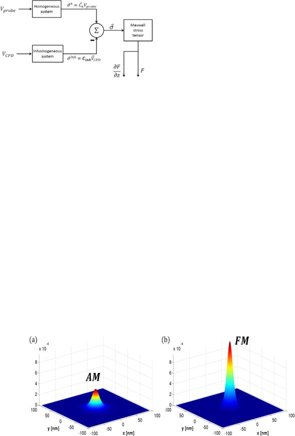
probe, the vector Ch is the capacitance between the probe’s surface elements and a grounded surface and the matrix Cinh describes the mutual capacitance between every probe surface element and sample surface element pair. The force (F) and force-gradient (@F=@z) distributions on the probe are obtained by inserting E into the Maxwell stress tensor. A flow chart of the electrostatic model is delineated in figure 3. The AM-PSF and FM-PSF are then obtained by setting the feedback bias VDC, which satisfies F! D 0 and @F!=@z D 0, respectively, where ! indicates the KPFM modulation frequency. Figure 4 shows examples of two-dimensional AMand FM-PSFs.

When scanning an equipotential substrate, the KPFM measures the exact surface potential. Therefore, integration of the PSFs over the entire x–y surface must be equal to one. Summations over the AM-PSF and the FM-PSF components in figure 4 are 0.5856 and 0.9999, respectively. The FM-PSF converges to a total sum of 1, as expected. However, due to the long-range electrostatic forces, integration over the AM-PSF yields a smaller value since computational limitations do not allow performing simulations on an infinite sample. Instead, we considered a finite square sample .192 nm 192 nm/, which is sufficient to contain merely 59% of the AM-PSF. Therefore, the AM-PSF must be extrapolated beyond the measurement boundaries in order to obtain the full system response. The extrapolation is described in the appendix. We show that extrapolation performed on an AM-PSF generated

for	a probe at a tip–sample distance of 2 nm increases
the	summation over	the PSF	components from	0.831 89
(for	5 m 5 m	area) to	0.998 24 (for 0:3	mm

0:3 mm area). It should also be noted that summation over AM-PSF components approaches 1 as the tip–sample distance decreases, since most of the force stems from the tip apex sphere, and by lowering the tip–sample distance the sphere ‘sees’ more of the sample and less of the truncated area.

Alternatively, deconvolution can be performed by subtracting the average CPD of the sample, Vsub, which is usually the CPD value of the substrate outside the scan area. The reconstruction is then performed using (the mathematical

Figure 4. Two-dimensional PSFs of (a) AM-KPFM and (b) FM-KPFM. The PSFs were calculated for the same probe geometry and tip–sample distance (5 nm).

3

Nanotechnology 24 (2013) 295702

G Cohen et al

Figure 5. (a) Cross-section of a tip with a spherical apex radius R, cone length l, and half aperture angle 0, connected to a cantilever with length, width and thickness of L; W and t, respectively. (b)

Cross-section of a probe-sample system composed from a cantilever tilted by degrees towards the sample and a tip–sample distance of d. All the analyses were carried out using the parameter values:

L D 225 m, W D 40 m, t D 7 m, l D 13 m, R D 30 nm and0 D 17:5 .

formation is detailed in the appendix):

VDC Vsub

|{z }

Deconvolution input

D	h.VCPD Vsub/ XPSF i ~						PSF	(7)
							PSF
	|		{z		}		P
		Deconvolution output

P

where PSF denotes summation over the PSF.

3.2. Comparison between AMand FM-PSF

The differences between the minimum force and forcegradient conditions presented earlier yield two distinct PSFs with different characteristics. The probe under study is composed from a conical tip ending with a spherical cap that is kept at a constant tip–sample distance and a cantilever tilted relative to the sample surface. The geometric parameters of the probe are presented in figure 5(a). We define as the tilt angle and d as the tip–sample distance (figure 5(b)).

Figure 6 shows the effect of the cantilever on the AMand FM-PSFs for two different tip–sample distances with and without the cantilever, represented by the solid and dashed lines, respectively. At a tip–sample distance of d D 5 nm the peak value of the full probe AM-PSF is reduced by a factor of 1.65 compared to the tip-only AM-PSF (figure 6(a)), whereas the FM-PSF is left unchanged in the presence of the cantilever (figure 6(c)). For a tip–sample distance of d D 30 nm the cantilever contributes 45% of the homogeneous force (the force generated from the homogeneous system), which attenuates the AM-PSF peak by a factor of 4.12 (figure 6(b)), whereas the FM-PSF peak value is slightly decreased by 15% (figure 6(d)). This small attenuation of the full probe (tip C cantilever) FM-PSF is because of a portion of homogeneous force-gradient (25%) which stems from the tilted tip cone and not from the cantilever. The horizontal arrows, which represent the full width at half maximum

Figure 6. AMand FM-PSFs simulated for two different tip–sample distances d with and without the cantilever, represented by the solid (red) and dashed (blue) lines, respectively. (a) AM-PSF for d D 5 nm. (b) AM-PSF for d D 30 nm. (c) FM-PSF for d D 5 nm. (d) FM-PSF for d D 30 nm. The horizontal lines represent the FWHM of the PSFs—solid lines for the full probe (tip C cantilever) and dashed lines for the tip only. The simulations were performed with a tilt angle of D 20 for the full probe.

4

Nanotechnology 24 (2013) 295702

G Cohen et al

Figure 7. (a) Full width at half maximum of both AM-PSF (dashed line) and FM-PSF (solid line) as a function of the tip–sample distance.

(b)PSF peak value (maximal PSF value) as a function of the tip–sample distance for AM-PSF (dashed line) and FM-PSF (solid line).

(c)and (d) show small sections from (a) and (b) (illustrated by dashed rectangles), respectively, demonstrating the PSFs FWHM and peak value at conventional tip–sample distances.

(FWHM) for the four cases, demonstrate that the cantilever hardly affects the measurement resolution.

Figure 7(a) shows the FWHM dependence on the tip–sample distance for both AM-PSF (dashed line) and FM-PSF (solid line). The FM-PSF has a smaller FWHM than AM-PSF for all tip–sample distances, which indicates a superior resolution of FM-KPFM over AM-KPFM. Figure 7(b) shows the PSF peak value (maximal PSF value) as a function of the tip–sample distance. It is observed that the FM-PSF (solid line) has a much higher peak value than the AM-PSF (dashed line). For example, at a tip–sample distance of 30 nm, which is frequently used in ambient KPFM, the FM-PSF peak is an order of magnitude higher than that of the AM-PSF. Since the contrast of the CPD images has a correlation to the PSF peak value, the contrast is superior in FM-KPFM as compared to AM-KPFM. The PSFs FWHM and peak at conventional tip–sample distances (1–30 nm) are presented in figures 7(c) and (d), respectively.

Figure 8 presents the summation over the PSFs as a function of the tip–sample distance for a 192 nm 192 nm sample area. The left (right) axis corresponds to the AM-PSF (FM-PSF). It is observed that the summation over the AMPSF decreases rapidly, whereas the summation over the FMKPFM is above 90% for conventional tip–sample distances (1–50 nm). We conclude that AM-KPFM measurements

are	extremely sensitive to the tip–sample distance and
are	highly affected by the background	CPD, especially
for	tip–sample distances larger than 10	nm. In contrast,

FM-KPFM measurements demonstrate little dependence of the measured KPFM signal on the tip–sample distance, since

Figure 8. Summation over the AM-PSF (left axis) and FM-PSF (right axis) versus the tip–sample distance. All PSFs were simulated for a 192 nm 192 nm sample area.

most of the measured force-gradient stems from the area beneath the tip. Our results are in good agreement with the measurements of Ziegler et al [3], which demonstrated that tip–sample distance has a weak effect on the measured FM-KPFM signal whereas the dependence of AM-KPFM measurements on the tip–sample distance is prominent.

3.3. Effective PSFs

In KPFM measurements performed with the single pass technique, the Kelvin probe controller minimizes the oscillations of the cantilever’s second resonance frequency (for AM) or the oscillations at f0 fmod (for FM), where f0 and fmod are the cantilever’s first resonance and modulation

5