2013 CFA Level 1 - Book 5

Study Session 16

Cross-Reference to CFA Institute Assigned Reading #57 - Yield Measures, Spot Rates, and Forward Rates

1 1 . B Spot rates: 51 = 5.5%.

52 = [(1 .055)(1 .0763)]112 - 1 = 6.56%

53 = [(1 .055)(1 .0763)(1.1218)] 113 - 1 = 8.39%

54 = [(1 .055)(1 .0763)(1.1218)(1. 155)] 114 - 1 = 10.13%

Bond value:	-94.79
N = 1; FV = 100; I/Y = 5.5; CPT --+ PV=
N = 2; FV = 100; I/Y = 6.56; CPT --+ PV=	-88.07
N = 3; FV = 100; I/Y = 8.39; CPT --+ PV=	-78.53
N = 4; FV = 1,100; 1/Y = 10.13; CPT --+ PV=	-747.77

Total: $1,009.16

12. A Find the spot rate for 3-year lending:

53 = [(1 .055)(1 .0763)(1.1218)]113 - 1 = 8.39%

Value of the bond: N = 3; FV = 1,000; 1/Y = 8.39; CPT--+PV = -785.29

or	$1'000	= $785.05
	(1.055)(1.0763)(1.1218)

13. C Ifthe yield curve is flat, the nominal spread and the Z-spread are equal. Ifthe bond is option-free, the Z-spread and OAS are equal.

14.C A Treasury bond is the best answer. The Treasury spot yield curve will correctly price an on-the-run Treasury bond at its arbitrage-free price, so the Z-spread is zero.

15. A The Z-spread will be greater than the nominal spread when the spot yield curve is upward sloping.

ANSWERS - CHALLENGE PROBLEMS

1. The three sources ofreturn are coupon interest payments, recovery ofprincipal/capital gain or loss, and reinvestment income.

Coupon interestpayments: 0.07 I 2 x $100,000 x 6 = $21,000

Recovery ofprincipal/capitalgain or loss: Calculate the sale price of the bond:

N = (10 - 3) X 2 = 14; 1/Y = 6.9 I 2 = 3.45; PMT = 0.07 I 2 X 100,000 = 3,500;

FV = 100,000; CPT --+ PV = -100,548

Capital gain = 100,548 - 92,800 = $7,748

Reinvestment income: We can solve this by treating the coupon payments as a 6-period annuity, calculating the future value based on the semiannual interest rate, and subtracting the coupon payments. The difference must be the interest earned by reinvesting the coupon payments.

N = 3 x 2 = 6; IIY = 5 I 2 = 2.5; PV = 0; PMT = -3,500; CPT --+ FV = $22,357

Reinvestment income = 22,357 - (6 x 3,500) = $ 1,357

Page 130

©2012 Kaplan, Inc.

The following is a review oftheAnalysis ofFixed Income Investments principles designed to address the learning outcome statements set forth by CFA Institute. This topic is also covered in:

INTRODUCTION TO THE MEASUREMENT OF INTEREST RATE RISK

Study Session 16

EXAMFOCUS

This topic review is about the relation ofyield changes and bond price changes, primarily based on the concepts of duration and convexity. There is really nothing in this study session that can be safely ignored; the calculation of duration, the use of duration, and the limitations of duration as a measure of bond price risk are all important. You should work to understand what convexity is and its relation to the interest rate risk of fixed­ income securities. There are two important formulas: the formula for effective duration and the formula for estimating the price effect of a yield change based on both duration and convexity. Finally, you should get comfortable with how and why the convexity of a bond is affected by the presence of embedded options.

LOS 58.a: Distinguish between the full valuation approach (the scenario analysis approach) and the duration/convexity approach for measuring interest rate risk, and explain the advantage of using the full valuation approach.

CPA® Program Curriculum, Volume 5, page 556

The full valuation or scenario analysis approach to measuring interest rate risk is based on applying the valuation techniques we have learned for a given change in the yield curve (i.e., for a given interest rate scenario). For a single option-free bond, this could be simply, "if the YTM increases by 50 bp or 100 bp, what is the impact on the value of the bond?" More complicated scenarios can be used as well, such as the effect on

the bond value of a steepening of the yield curve (long-term rates increase more than short-term rates). If our valuation model is good, the exercise is straightforward: plug in the rates described in the interest rate scenario(s), and see what happens to the values of the bonds. For more complex bonds, such as callable bonds, a pricing model that incorporates yield volatility as well as specific yield curve change scenarios is required to use the full valuation approach. If the valuation models used are sufficiently good, this is the theoretically preferred approach. Applied to a portfolio of bonds, one bond at a time, we can get a very good idea of how different interest rate change scenarios will affect the value of the portfolio. Using this approach with extreme changes in interest rates is called stress testing a bond portfolio.

The duration/convexity approach provides an approximation of the actual interest rate sensitivity of a bond or bond portfolio. Its main advantage is its simplicity compared to the full valuation approach. The full valuation approach can get quite complex and time consuming for a portfolio of more than a few bonds, especially if some of the bonds have more complex structures, such as call provisions. As we will see shortly, limiting our scenarios to parallel yield curve shifts and settling for an estimate of interest rate risk

Page 134

©2012 Kaplan, Inc.

Study Session 16 Cross-Reference to CFA Institute Assigned Reading #58 - Introduction to the Measurement ofInterest Rate Risk

allows us to use the summary measures, duration, and convexity. This greatly simplifies the process of estimating the value impact of overall changes in yield.

Compared to the duration/convexity approach, the full valuation approach is more precise and can be used to evaluate the price effects of more complex interest rate scenarios. Strictly speaking, the duration-convexity approach is appropriate only for estimating the effects of parallel yield curve shifts.

Example: The full valuation approach

Consider two option-free bonds. Bond X is an 8% annual-pay bond with five years to maturity, priced at 108.4247 to yield 6% (N = 5; PMT = 8.00; FV = 100; 1/Y = 6.00%; CPT PV =-108.4247).

Bond Y is a 5% annual-pay bond with 15 years to maturity, priced at 8 1 .7842 to yield 7%.

Assume a $ 1 0 million face-value position in each bond and two scenarios. The first scenario is a parallel shift in the yield curve of+50 basis points, and the second scenario is a parallel shift of+ 100 basis points. Note that the bond price of 108 .4247 is the price per $100 ofpar value. With $ 1 0 million ofpar value bonds, the market value will be

$ 10.84247 million.

Answer:

The full valuation approach for the two simple scenarios is illustrated in the following figure.

The Full ValuationApproach

Market Value of

Scenario	Yield	BondX	Bond Y	Portfolio	Portfolio
		(in miiiions}	(in miiiions}		Value %
Current	+0 bp	$10.84247	$8. 17842	$ 19.02089
1	+50 bp	$10.62335	$7.79322	$ 18.41657	-3.18%
2	+100 bp	$10.41002	$7.43216	$17.84218	-6.20%

N = 5 ; PMT = 8; FV = 1 00; 1/Y = 6% + 0.5%; CPT PV = -1 06.2335

N= 5; PMT = 8; FV = 1 00; 1/Y = 6% + 1%; CPT PV = - 104. 1 002

N= 1 5 ; PMT = 5; FV = 1 00; 1/Y = 7% + 0.5%; CPT PV = -77.9322

N= 15; PMT = 5; FV = 1 00; 1/Y = 7% + 1 %; CPT PV = -74.3216

Portfolio value change 50 bp: ( 1 8.4 1 657 - 19.02089) I 19.02089 = -0.03 177 = -3. 1 8%

©2012 Kaplan, Inc.

Page 135

Study Session 16 Cross-Reference to CFA Institute Assigned Reading #58 - Introduction to the Measurement ofInterest Rate Risk

First, note that the price-yield relationship is negatively sloped, so the price falls as the yield rises. Second, note that the relation follows a curve, not a straight line. Because the curve is convex (toward the origin), we say that an option-free bond has positive convexity. Because of its positive convexity, the price of an option-free bond increases

more whenyields fall than it decreases whenyields rise. In Figure 1 , we have illustrated

that, for an 8%, 20-year option-free bond, a 1% decrease in the YTM will increase the price to 1 1 0.67, a 10.67% increase in price. A 1 % increase in YTM will cause the bond value to decrease to 90.79, a 9.22% decrease in value.

If the price-yield relation were a straight line, there would be no difference between the price increase and the price decline in response to equal decreases and increases in yields. Convexity is a good thing for a bond owner; for a given volatility of yields,

price increases are larger than price decreases. The convexity property is often expressed by saying, "a bond's price falls at a decreasing rate as yields rise." For the price-yield relationship to be convex, the slope (rate of decrease) of the curve must be decreasing as we move from left to right (i.e., towards higher yields).

Note that the duration (interest rate sensitivity) of a bond at any yield is (absolute value of) the slope of the price-yield function at that yield. The convexity of the price-yield relation for an option-free bond can help you remember a result presented earlier, that the duration of a bond is less at higher market yields.

Callable Bonds, Prepayable Securities, and Negative Convexity

With a callable or prepayable debt, the upside price appreciation in response to decreasing yields is limited (sometimes called price compression). Consider the case of a bond that is currently callable at 102. The fact that the issuer can call the bond at any

time for $ 1 ,020 per $ 1 ,000 of face value puts an effective upper limit on the value of the bond. As Figure 2 illustrates, as yields fall and the price approaches $ 1 ,020, the price­ yield curve rises more slowly than that of an identical but noncallable bond. When the price begins to rise at a decreasing rate in response to further decreases in yield, the price­ yield curve bends over to the left and exhibits negative convexity.

Thus, in Figure 2, so long as yields remain below levely', callable bonds will exhibit negative convexity; however, at yields above levely', those same callable bonds will exhibit positive convexity. In other words, at higher yields the value of the call options becomes very small so that a callable bond will act very much like a noncallable bond. It is only at lower yields that the callable bond will exhibit negative convexity.

©2012 Kaplan, Inc.

Page 137

Study Session 16 Cross-Reference to CFA Institute Assigned Reading #58 - Introduction to the Measurement ofInterest Rate Risk

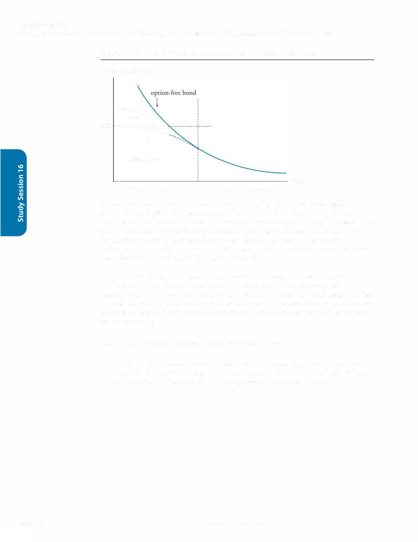
Figure 3: Comparing the Price-Yield Curves for Option-Free and Putable Bonds

Price

putable bond

-.. /

---- ....._______

option-free bond

Yield

y'

In Figure 3, the price of the putable bond falls more slowly in response to increases in yield above y' because the value of the embedded put rises at higher yields. The slope of the price-yield relation is flatter, indicating less price sensitivity to yield changes (lower duration) for the putable bond at higher yields. At yields below y', the value of the put is quite small, and a putable bond's price acts like that of an option-free bond in response to yield changes.

LOS 58.d: Calculate and interpret the effective duration of a bond, given information about how the bond's price will increase and decrease for given changes in interest rates.

CPA® Program Curriculum, Volume 5, page 569

In our introduction to the concept of duration, we described it as the ratio of the percentage change in price to change in yield. Now that we understand convexity, we know that the price change in response to rising rates is smaller than the price change in response to falling rates for option-free bonds. The formula we will use for calculating the effective duration of a bond uses the average of the price changes in response to equal increases and decreases in yield to account for this fact. Ifwe have a callable bond that is trading in the area of negative convexity, the price increase is smaller than the price decrease, but using the average still makes sense.

©20 12 Kaplan, Inc.

Page 139