SPWLA-2013-RR

SPWLA 54th Annual Logging Symposium, June 22-26, 2013

QUANTIFYING ORGANIC POROSITY FROM LOGS

James Galford, John Quirein, Donald Westacott, and James Witkowsky, Halliburton

Copyright 2013, held jointly by the Society of Petrophysicists and Well Log Analysts (SPWLA) and the submitting authors. This paper was prepared for presentation at the SPWLA 54th Annual Logging Symposium held in New Orleans, Louisiana, June 22-26, 2013.

ABSTRACT

Organic, or kerogen, porosity is created during the thermal maturation of organic matter, which can include expulsion of hydrocarbons from the solid kerogen framework. Recent work done on core samples with highmagnification electron microscopy has shown that organic porosity can be nonnegligible. In fact, it is believed the amount of organic porosity is an important factor in the sustainable production that occurs from source rock reservoirs following an initial rapid decline. Moreover, organic porosity contributes to the total hydrocarbon storage capacity of source rock reservoirs. Thus, quantification of organic porosity is a valuable parameter in reservoir assessment and simulation.

Laboratory measurements of organic porosity are expensive, time-consuming, and done on a scale that does not represent the bulk rock. Because of this, relying on laboratory measurements of organic porosity is not practical for routine source rock reservoir evaluations. This paper presents a method for determining organic porosity from well logs so that a more detailed reservoir evaluation can be made. The process is built around fundamental concepts of thermal maturation and conversion of organic matter into hydrocarbons and can be applied to all types of kerogen.

Example logs from Haynesville and Eagle Ford source rock reservoirs are presented to demonstrate how the process can be used to obtain a breakout of formation porosity into organic and nonorganic (porous mineral) fractions. The process is easily adapted to other source rock reservoirs. In addition, the log-derived organic porosity from this procedure can be used in downstream source rock reservoir simulators to obtain better estimates of production and recoverable hydrocarbons.

INTRODUCTION

Activity and interest in unconventional source rock reservoirs has grown steadily over the past few years and great strides have been made to develop methods and technology to exploit these previously untapped resources. Along with the heightened focus on bringing new energy resources online, a parallel effort by operators, service companies, and academia to understand the mechanisms that make these nontraditional reservoirs commercially viable has intensified. While much remains to be learned, progress is being made, and the techniques discussed here represent one small step toward achieving greater insight into evaluating the producibility of source rock reservoirs.

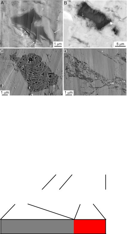
Recent Scanning Electron Microscopy (SEM), Transmission Electron Microscopy (TEM), and Focused Ion Beam/Scanning Electron Microscopy (FIB/SEM) studies (Loucks, 2009 and Curtis, 2011) have revealed nanometer pore systems within organic-rich rocks that provide new insight into observed production histories in source rock reservoirs. These discoveries show that source rock reservoirs are comprised of three types of porosity: conventional intergranular, natural fracture, and organic, or kerogen porosity. Figure 1 shows example SEM images of organic matter in lowand high-maturity samples. Images from the low-maturity samples show few or no nanopores. In contrast, the high-maturity samples contain well-developed intragranular kerogen porosity. The correlation between thermal maturity and the abundance of intragranular pores in organic matter suggests the formation of organic porosity is linked to the maturation and conversion of kerogen into hydrocarbons (Loucks, 2009).

1

SPWLA 54th Annual Logging Symposium, June 22-26, 2013

Fig. 1 A) Organic matter with vitrinite reflectance < 0.5%. B) Kerogen maceral with no apparent nanopores and vitrinite reflectance ~0.52%. C) Well-developed kerogen porosity in a Barnett Shale sample whose vitrinite reflectance ~ 1.6. D) Disseminated organic matter with associated nanopores. Images from Loucks et al., 2009.

Intragranular kerogen, or organic, porosity is an additional effective porosity component in source rock reservoirs that is not present in conventional reservoir rocks as shown in Figure 2. The organic porosity system in source rock reservoirs is unique compared to conventional porosity associated with porous minerals. Because it is created by thermal maturation and conversion of organic matter into hydrocarbons, organic porosity is oil-wet unlike most instances of conventional porosity. The creation of organic porosity is strongly influenced by the thermal history of the reservoir. The amount created in the bulk rock is proportional to the present-day solid kerogen volume. Thus, organic porosity contributes to the total reservoir hydrocarbon storage capacity and may be the major storage mechanism in some productive source rock reservoirs.

Conventional Reservoir

Non-clay

Dry-clay

Clay-bound

Capillary-bound

&

Gas / Oil

Minerals

Minerals

Water

Movable Water

Total Porosity

Source Rock Reservoir

Effective Porosity

Non-clay

Solid

Dry-clay

Clay-bound

Capillary-bound

Kerogen

&

Porosity

Gas / Oil

Minerals

Kerogen

Minerals

Water

Movable Water

Gas / Oil

Porous Kerogen

Intragranular Porosity

Solid Kerogen Associated

With Kerogen, Φk

Fig. 2 Intragranular kerogen porosity introduces a new component of effective porosity not present in conventional reservoirs.

Organic porosity may explain the long-term production profile observed for several source rock reservoirs (Figure 3). One hypothesis is the rapid initial decline is associated with the drawdown of conventional intergranular and

2

SPWLA 54th Annual Logging Symposium, June 22-26, 2013

natural fracture porosity that is quickly depleted. After the conventional pore system is depleted, the reservoir continues to produce from the organic porosity at a significantly lower rate and also at a slower rate of decline. An essential part of this hypothesis is that micro fractures, created during hydrocarbon expulsion, connect the organic porosity to the conventional porosity production network and limit production from it. Several researchers are working to broaden the understanding of production mechanisms in source rock reservoirs and develop robust reservoir simulators.

	Conventional Intergranular Porosity Production
Rate	Organic Porosity Production
	Total Production
Production
	Time

Fig. 3 Hypothetical source rock reservoir production decline curve. Total production is comprised of contributions from intergranular matrix porosity and intragranular organic porosity.

Therefore, based on current thinking and the reasons previously discussed, organic porosity is a reservoir parameter which is important for simulating well performance and assessing recoverable reserves. The techniques presented in this paper can be used to quantify organic porosity from logs so that more detailed reservoir evaluations can be made. In addition, organic porosity volumes computed from logs can be used by downstream source rock reservoir simulators to improve predictions of production and recoverable hydrocarbons.

ORGANIC POROSITY FROM THERMAL TRANSFORMATION

The framework to calculate the organic porosity associated with thermally matured organic matter is based on a mass balance relationship involving the amount of convertible carbon and thermal maturity (Modica, 2012). The kerogen porosity created in the formation, k, is given by:

k TOCo Cc k TR b

k

(1)

where TOCo is the initial total organic carbon weight fraction, Cc is the weight fraction of carbon that is convertible, k is a scale factor that represents the kerogen mass equivalent of a convertible carbon mass, TR is the transformation ratio, b is the formation bulk density, and k is the density of kerogen. Although rigorous, Equation 1 is difficult to use with logs because it depends on the initial total organic carbon weight fraction, and log responses are influenced by present-day organic content. An expression compatible with multitool log analysis techniques can be constructed by recognizing that formation kerogen porosity is proportional to present-day solid kerogen volume. This leads to a relationship in terms of the porosity associated with porous kerogen, Φk, and solid kerogen volume, Vsk:

k			Φk	Vsk .	(2)
			Φk
	1

Φk can be estimated by normalizing Equation 1 with respect to the initial kerogen volume, Vki:

Φ			k		TOCo Cc k TR b	k	C	k TR TOC
	k
		Vki			TOCo TOCk b k		c	k
								(3)

where TOCk is the weight fraction of carbon in kerogen. Modica (2012) calculated the scale factor, k, by assuming 95% of the initial total organic carbon is from kerogen and a convertible carbon mass represents 85% of a

3

SPWLA 54th Annual Logging Symposium, June 22-26, 2013

convertible kerogen mass so that k ~ 0.95/0.85 or ~1.118. Chemical analyses of kerogen material (Yen, 1976) suggests the weight fraction of carbon in immature kerogen is ~ 0.773. Thus, the porosity associated with kerogen can be predicted from the carbon lability and transformation ratio.

Log analysis systems that use probabilistic error-minimization techniques to derive formation volumes from multiple log responses are well-suited to calculating formation kerogen porosity from Equation 2. To achieve this, the tool response equations are adapted to follow the source rock reservoir model shown in Figure 2. For example, the density log response would be cast in a form similar to:

b Vpmw w Vpmh Vpkh h Vcbw cbw Vdc dc Vsk sk Vncm ncm

(4)

where Vpmw, Vpmh, Vpkh, Vcbw, Vdc, Vncm, and Vsk are the porous mineral water, porous mineral hydrocarbon, porous kerogen hydrocarbon, clay-bound water, dry clay, non-clay mineral, and solid kerogen bulk volumes, respectively,

and ρw, ρh, ρcbw, ρdc, ρncm, and ρsk are the bulk densities of water, hydrocarbon, clay-bound water, dry clay, non-clay mineral, and solid kerogen. Equation 4 can be simplified by using Equation 2 for the porous kerogen hydrocarbon

volume:

				Φ		h
	b	Vpmw w Vpmh h Vcbw cbw Vdc dc	Vsk	k			sk	Vncm ncm	(5)
				1 Φk

so that the hydrocarbon-filled kerogen pore volume does not have to be solved for explicitly, and the formation hydrocarbon volume, Vh, is given by:

Vh	Vpmh			Φk	Vsk .	(6)
				Φk
		1

An interesting consequence of Equation 6 is that the organic porosity represents a minimum hydrocarbon volume when the porous mineral hydrocarbon volume goes to zero. When a probabilistic error minimization log analysis technique is used, this boundary condition can be developed into an inequality constraint to restrict the available solution space.

CARBON LABILITY

Carbon lability is a characteristic of the organic matter originally deposited in the source rock. It is one of the parameters required to compute the porosity associated kerogen, which is required to derive organic porosity from logging measurements. A benefit of the growing interest in source rock reservoirs is that numerous laboratory studies have been conducted. Published results from some of these studies can be used to calculate the lability for several shale reservoirs (Jarvie, 2012). If immature rock samples are available, then Rock-Eval pyrolysis measurements can be used to derive the lability from:

Cc HIo 1000

(7)

where HIo represents the hydrogen index of the original material and is the carbon weight fraction in generated hydrocarbons. The carbon weight fraction in petroleum products formed from kerogen varies as the kerogen matures. However for our purposes the desired value is one that represents the gross elemental composition of the produced hydrocarbons. Values for typically fall in the range from 0.82 to 0.88 and a value of 0.85 is commonly used (Jarvie, 2012, and Dahl, 2004).

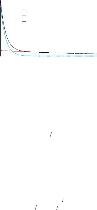
A crossplot of Rock-Eval pyrolysis S2 yields vs. total organic carbon weight percent from immature samples can be used to determine the initial hydrogen index as shown in Figure 4. The blue data points were obtained from Eagle Ford Shale core samples that had an average measured vitrinite reflectance, VRo, of 0.47%. The slope of the line determines the initial hydrogen index. In this example the indicated HIo = 664 and the corresponding lability for the Eagle Ford Shale from Equation 7 is Cc = 0.5645.

4

SPWLA 54th Annual Logging Symposium, June 22-26, 2013

Generation Potential (S2) (mg HC / g R)

100

90

80

70

60

S2 = 6.64 TOC (Wt. %)

50

40

30

20

10

0

0

2

4

6

8

10

12

14

16

18

20

Total Organic Carbon (Wt. %)

Fig. 4 Crossplot of pyrolysis S2 and total organic carbon data from immature Eagle Ford Shale samples.

Unfortunately, the Figure 4 graphical method cannot be used to determine HIo for the Haynesville Shale because immature samples are not available. In lieu of this, results for analog data from immature Kimmeridgian source rocks from the deepwater Gulf of Mexico (Jarvie, 2004) suggest HIo = 722 for the Haynesville Shale, which is equivalent to a carbon lability of 0.6137.

TRANSFORMATION RATIO

There are several techniques that can be applied to determine the transformation ratio required to calculate the porosity associated with kerogen. Because this parameter is tied to the thermal history of the reservoir, it will vary geographically in most instances. Therefore it should be evaluated on a well-by-well basis.

TR from core measurements - If Rock-Eval pyrolysis measurements on core samples are available, they can be used to derive TR after the carbon lability for the source rock reservoir is established. The idea is to calculate the average TR for the population of pyrolysis measurements by solving the equation:

	TR	1			TOC
			1			.	(8)
		Cc			TOCo

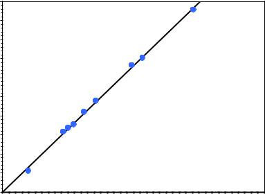
The original total organic carbon (TOC) can be found graphically by following the example shown in Figure 5. The nomograph is entered with the Rock-Eval S2 yield and present-day TOC after applying adjustments for inert carbon. To find TOCo, follow the red decomposition lines to the established iso-original hydrogen index line (HIo), shown in blue for the Eagle Ford Shale example. Then project a line vertically to the x-axis to obtain TOCo. Applying this procedure to the data point represented by the black circle symbol in Figure 5, S2 = 12.5 mg HC/gR and present-day TOC = 3.5 Wt. %, leads to TOCo = 5.6% for HIo = 664. The corresponding TR, calculated from Equation 8, is 0.66.

5

SPWLA 54th Annual Logging Symposium, June 22-26, 2013

	80
					900	800	700		600	500		400
	70
/ g R)	60
(mg HC
												300
	50
(S2)
Potential	40											200
	30
Generation
	20											100
	10
	0
	0	2	4	6	8	10		12	14	16	18	20

Total Organic Carbon (Wt. %)

Fig. 5 Nomograph to derive TOCo from core pyrolysis measurements (after Jarvie, 2012).

TR from vitrinite reflectance - Another method for obtaining the transformation ratio is to use another parameter that varies with the maturity of the organic source rock as a proxy for TR. Good examples are Rock-Eval Tmax, conodont color alteration index (CAI), and vitrinite reflectance (VRo). The link between the proxy and TR generally involves modeling the maturity of the source rock. Maturity modeling entails a number of steps, starting with construction of a burial and thermal history of the study area that is based on geological and geophysical data. The details of constructing a burial and thermal history for the reservoir are beyond the scope of this paper. However, useful working guides can be found in the literature (Waples, 1992). Burial and thermal histories in the public domain from academic and government studies may also be helpful.

After a satisfactory burial and thermal history is established, the next step is to model the generation of hydrocarbons by using a series of kinetics equations that simulate the cracking of kerogen (Braun, 1987, Tissot, 1987, and Sweeney, 1987). A system of parallel first-order Arrhenius equations of some form is generally used to calculate the conversion of kerogen over geological time. Kerogen cracking calculations require a distribution of activation energies. Several sets of distributions used previously are described in the literature (Tissot, 1987 and Waples, 1992). Researchers at Lawrence Livermore National Laboratory (LLNL) developed the frequently used set of activation energy distributions listed in Table 1 (Burnham, 1989). These are the distributions that we used to obtain the results in this paper. Hydrocarbon generation calculations can be performed using basin modeling software or they can be organized into a spreadsheet.

Vitrinite reflectance values corresponding to the calculated incremental hydrocarbon conversion were obtained by applying a different set of kinetics equations to the established burial and thermal history. We used the EASY%Ro method (Sweeney, 1990) for the Eagle Ford and Haynesville Shale examples discussed in the following text. To obtain a valid correlation between vitrinite reflectance and TR, the results from the EASY%Ro calculations must be correlated with hydrocarbon generation calculations using a set of activation energies appropriate for the reservoir kerogen type (Waples, 1998).

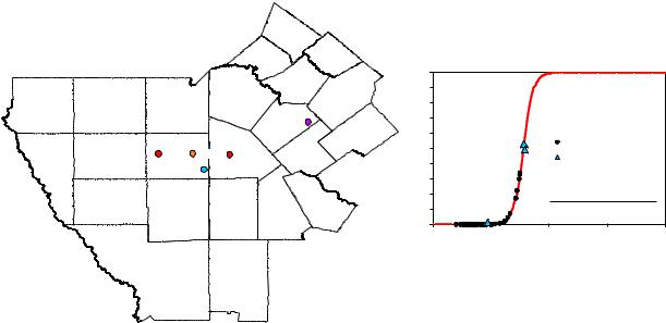
We found burial history models in the public domain for the H. A. Halff and B. M. Winkler wells in South Texas that are approximately located as shown in Figure 6 (Cardneaux, 2012, and Condon, 2006). Figure 7 shows the burial and temperature histories for each well with calculated TR and vitrinite reflectance histories obtained by applying the aforementioned kinetics calculations for Type II kerogen. A least-squares fit was performed on the combined results from both wells to obtain the VRo-TR correlation represented by the red curve in the right-hand panel of Figure 6.

6

SPWLA 54th Annual Logging Symposium, June 22-26, 2013

Table 1. LLNL hydrocarbon generation activation energy distributions.

Kerogen Type	Type I	Type II	Type III
Frequency Factors(s-1)	5.073e13	3.012e13	1.617e13
Energy (kcal/mole)	Fraction at given energy
48	0.07		0.04
49		0.05
50		0.20	0.14
51		0.50
52	0.93	0.20	0.32
53		0.05
54			0.17
56			0.13
60			0.10
64			0.07
68			0.03

	Hays
Comal	Caldwell

				Guadalupe
			Bexar	Gonzales
Kinney	Uvalde	Medina
				VRo = 0.785
				Wilson
				DeWitt
		H. A. Halff #1	Atascosa
				Karnes
	Zavala	Frio	VRo = 0.47
			B. M. Winkler #1
Maverick		VRo = 0.79
	Dimmit			Bee
		La Salle	McMullen	Live Oak

Webb

Duval

Transformation Ratio

1
0.9
0.8
0.7
0.6
0.5			Kinetics Simulations
			Average Core (3 Wells)
0.4
0.3
0.2			1
0.1		TR 1 97723655e 23.6366VRo
0
0.00	0.50	1.00	1.50	2.00

Vitrinite Reflectance (%)

Fig. 6 Eagle Ford Shale well locations. Measured vitrinite reflectance (VRo) and transformation ratios derived from pyrolysis data agree with the results from kinetics modeling.

Pyrolysis and vitrinite reflectance measurements performed on core samples were available for three Eagle Ford Shale wells. Samples from one well contained immature organic matter and samples from the other two wells were of intermediate maturity. TR values derived from the core pyrolysis data and the measured VRo values from all three wells agree with the kinetics calculations. These results affirm the derived VRo-TR correlation can be used to obtain reasonable TR values from vitrinite reflectance measurements to calculate the porosity associated with kerogen.

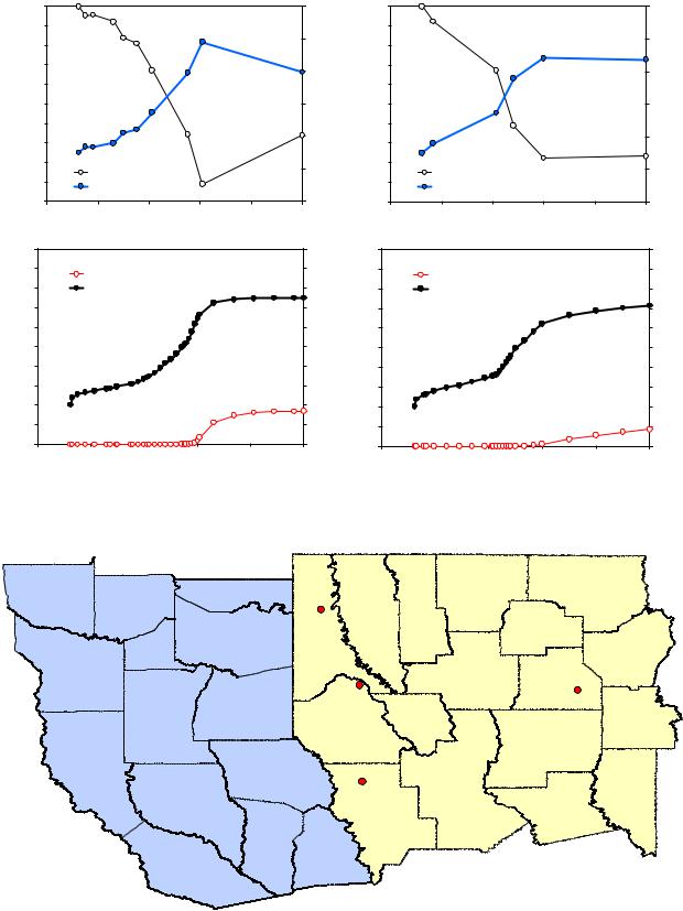
Maturity modeling calculations were also carried out for the Haynesville Shale and compared with measured vitrinite reflectance values and TR results derived from core pyrolysis measurements. We found burial history models for four wells that penetrated the Haynesville Shale in the public domain (Torsch, 2012). The wells are approximately located as shown in Figure 8. Haynesville Shale burial histories redrawn from the public domain models were used to calculate the kinetics results in Figure 9. The upper left panel in Figure 9 shows the Haynesville Shale burial history for each well and the upper right panel shows the reservoir temperature histories. Transformation ratio results from Type II kerogen hydrocarbon generation kinetics calculations are presented in the lower left panel of Figure 9 and the corresponding kinetics vitrinite reflectance simulations appear in the lower right panel.

7

SPWLA 54th Annual Logging Symposium, June 22-26, 2013

	0
	1000
	2000
	3000
(ft)	4000
Depth	5000
	6000
	7000
	8000
		Burial Depth
	9000	Temperature
	10000
	100	80	60	40	20	0

300			0					300
			1000
250			2000					250
200	Temperature (degF)		3000					200	Temperature (degF)
		Depth (ft)	4000
150			5000					150
			6000
100			7000					100
50			8000					50
				Burial Depth
			9000	Temperature
0			10000					0
			100	80	60	40	20	0

Time (my)

Time (my)

	2					1			2
	1.8	Kinetics TR				0.9			1.8
							(%)
	1.6	Kinetics VRo				0.8			1.6
	1.4					0.7	Vitrinite Reflectance		1.4
Kinetics TR	1.2					0.6		Kinetics TR	1.2
	1					0.5			1
	0.8					0.4			0.8
	0.6					0.3	Kinetics		0.6
	0.4					0.2			0.4
	0.2					0.1			0.2
	0					0			0
	100	80	60	40	20	0

					1
	Kinetics TR				0.9
						(%)
	Kinetics VRo				0.8
					0.7	Reflectance
					0.6
					0.5
						Vitrinite
					0.4
					0.3	Kinetics
					0.2
					0.1
					0
100	80	60	40	20	0

Time (my)

Time (my)

Fig. 7 Top panels show reconstructed burial and thermal histories for the Eagle Ford Shale in two South Texas wells (after Cardneaux, 2012 and Condon, 2006). Bottom panels show TR and vitrinite reflectance histories calculated from kinetics simulations for Type II kerogen.

Wood		Marion			Claiborne	Union
	Upshur			Bossier	Webster
				Gish #1
				Caddo		Lincoln
		Harrison
	Gregg					Ouachita
Smith					Bienville
						Jackson
				Foster #1		Tremont #C1
		Panola
	Rusk				Red River	Caldwell
				De Soto
						Winn
Cherokee			Shelby
				Cates #1
					Natchitoches
						La Salle
	Nacogdoches					Grant
				Sabine

San Augustine

Sabine

Angelina

Fig. 8 Burial histories for four North Louisiana wells, shown in red, were used to derive kinetics VRo and TR values for the Haynesville Shale.

8

SPWLA 54th Annual Logging Symposium, June 22-26, 2013

	0						400
	2000						350
					Tremont #C1
	4000				Foster #1		300
						Temperature (degF)
Depth (ft)	6000				Gish #1		250
					Cates #C1
	8000						200
	10000						150
							100
	12000
							50
	14000
							0
	150	120	90	60	30	0

150

120

90

60

30

0

Time (my)

Time (my)

	1						2.50
	0.9
	0.8					(%)	2.00
	0.7					Vitrinite Reflectance
Kinetics TR	0.6						1.50
	0.5
	0.4						1.00
	0.3					Kinetics
	0.2						0.50
	0.1
	0						0.00
	150	120	90	60	30	0

150

120

90

60

30

0

Time (my)

Time (my)

Fig. 9 Burial histories (after Torsch, 2012) and Type II kerogen kinetics maturity modeling results for the Haynesville Shale from four Northern Louisiana wells.

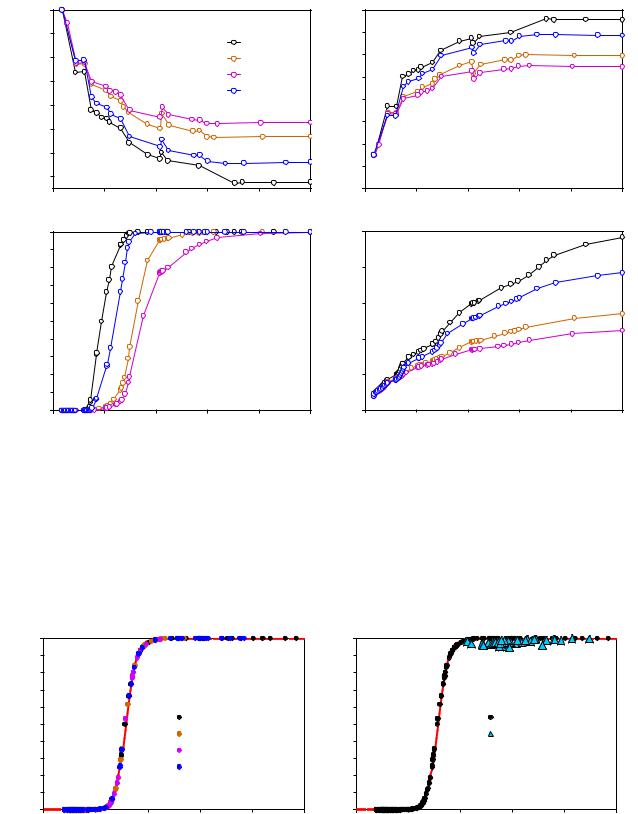
It is not obvious that the Haynesville Shale kinetics results can be represented by a single VRo-TR correlation based on a visual examination of the data in Figure 9. However, the combined results from all four wells, shown in Figure 10, show this to be the case. These results show the correlation between VRo and TR is not significantly affected by the rock’s thermal history for a given kerogen type. A universal VRo-TR correlation does not exist. VRo-TR correlations created from LLNL and EASY%Ro kinetics calculations are only valid for the three standard kerogen types identified in Table 1. Correlations for other kerogen types or vitrinite must be established empirically (Waples, 1998). However these results demonstrate that after the relationship is determined for a given kerogen, it is valid for all geological histories and heating rates.

Transformation Ratio

1							1
0.9							0.9
0.8						Ratio	0.8
0.7							0.7
0.6			Cates #C1			Transformation	0.6			Assumed HIo = 408.4
0.5			Tremont #C1				0.5			Kinetics Simulations
										Average Core (~40 Wells)
0.4			Foster #1				0.4
			Gish #1
0.3							0.3
0.2							0.2
0.1							0.1
0							0
0.00	0.50	1.00	1.50	2.00	2.50		0.00	0.50	1.00	1.50	2.00	2.50
		Vitrinite Reflectance (%)							Vitrinite Reflectance (%)

Fig. 10 Combined maturity modeling results for the Haynesville Shale.

9

SPWLA 54th Annual Logging Symposium, June 22-26, 2013

The Haynesville Shale play is known to be a dry gas domain which implies complete or late-stage kerogen conversion. Data from a multiwell database of vitrinite reflectance and pyrolysis measurements were analyzed to calculate an average transformation ratio for each well. This was accomplished using the core pyrolysis yields with an assumed HIo of 408.4. The results are consistent with transformation ratios predicted by the kinetics correlation to VRo as shown in the right-hand panel of Figure 10.

ORGANIC POROSITY FROM SHALE CORE ANALYSIS

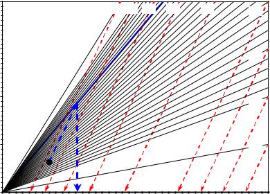
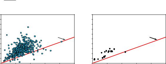
Results from the shale core analysis protocol (Gas Research Institute (GRI), 1996) can be used to obtain an empirical value for the porosity associated with kerogen. Figure 11 shows how we used the technique to obtain Φk for the Haynesville Shale by making a crossplot of gas-filled porosity from the shale core analyses vs. present-day kerogen volume. The data in Figure 11 are measurements from core samples taken from wells in Northeast Texas and Northern Louisiana. The technique relies on the relationship for the total volume of hydrocarbon (Equation 6— the volume of hydrocarbon in porous minerals plus the volume of hydrocarbon in porous kerogen). In source rock reservoirs the total volume of hydrocarbon approaches a minimum value when the volume of hydrocarbon in porous minerals approaches zero. Thus a trend near the lower-right edge of the data cluster represents the minimum hydrocarbon volume. The red line in Figure 11 represents the minimum hydrocarbon volume for the Haynesville Shale, and the porosity associated with kerogen is related to the slope so that:

Slope		Φk
		1 Φk .
	0.2						0.2
	0.18						0.18
(v/v)	0.16					(v/v)	0.16
	0.14						0.14
Porosity	0.12					Porosity	0.12
	0.1			Φk	0.3		0.1
filled						filled
	0.08						0.08
Gas-	0.06					Gas-	0.06
	0.04						0.04
	0.02						0.02
	0						0
	0	0.05	0.1	0.15	0.2	0.25	0

Kerogen Volume (v/v)

(9)

Φk 0.3

0.05

0.1

0.15

0.2

0.25

Kerogen Volume (v/v)

Fig. 11 GRI gas-filled porosity vs. present-day kerogen volume crossplots can be used to determine the porosity associated with kerogen. The left panel shows data from several Haynesville Shale wells. The right panel shows data from the Haynesville example log in this paper.

Accumulation of hydrocarbons in porous minerals displaces the results above the minimum hydrocarbon volume line. Thus, for this technique to be meaningful, it is important to have a population of data that includes points where the porous mineral hydrocarbon volume is zero. The right-hand crossplot in Figure 11 shows data from the Haynesville example well in this paper. In this case the data from the example well suggests that some porous mineral hydrocarbon is present in all but one of the data points. If only this data were considered, then it is possible that a steeper minimum hydrocarbon volume line would have been drawn, which corresponds to a larger Φk.

HIo and Cc values equivalent to the empirically derived Φk for the Haynesville shale, found by assuming TR = 1 and working with Equations 3 and 7, are HIo = 408.4 and Cc = 0.3471. These values are quite different from values based on immature Gulf of Mexico analogs of the Haynesville Shale (Jarvie, 2004). The equivalent Φk from Jarvie’s analog analysis would move the red line in Figure 11 to the upper-left of the data cloud in the left-hand panel. We do not know the cause of the discrepancy. However there are two possible explanations. One possibility is that the immature Gulf of Mexico analogs are invalid. Another possibility is that compaction of the kerogen macerals occurred during hydrocarbon generation and expulsion, which is not accounted for in Equation 1. We believe this is the most probable explanation and the empirical Φk is the correct value to use for the Haynesville Shale.

10