Interaction of the atmosphere with underlying surfaces.

Heat budgets

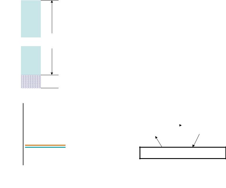
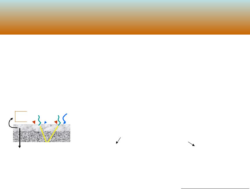
Active layer

Active layer is a layer of soil or water, within which temperature experiences diurnal and annual variations. The processes developing in this layer and those in laying above atmosphere are closely interrelated.

8-30 m Active layer

200-300 m

The active layer (especially that of the ocean) can greatly influence the
heat budget of the atmosphere.	2

Ma <200 km

M w 10 m

T

Ta

Tw

Ma M w 10000kg

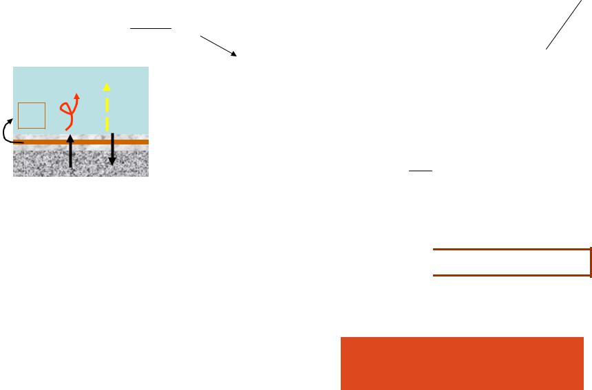
Ocean active layer 300 m depth= 30 atmospheres.

Air heat capacity at P=const is 4 times smaller than that of water. Therefore, the ocean input into vertical column heat content is 120 times larger than that of the atmosphere.

Tw 0,10 C Ta 120 C

In turn, ocean reacts on the wind causing waves and currents.

Air flows			Waves and
(wind)			currents

Structure of air flows

3

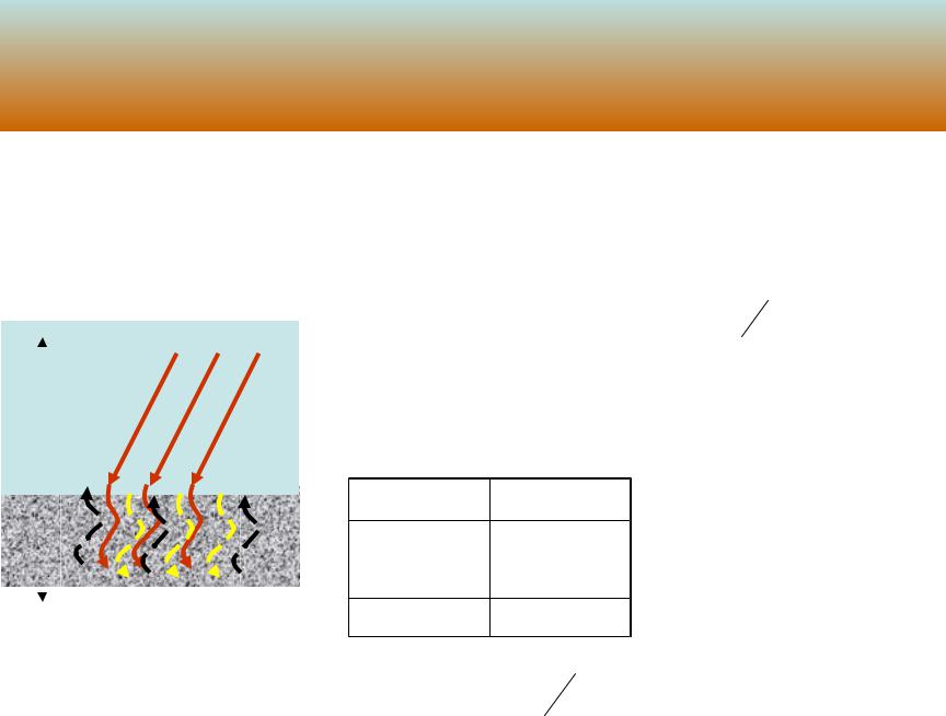
Soil heat conductivity equation

The energy arriving to the earth’s surface propagates to the depth of the soil due to molecular heat

	conductivity.
		QM		T	is soil heat conductivity
						coefficient W m K
	Z
		T 0 Q 0				T 0 Q 0
				M			M
			Soil				The soil heat
		Peat(торф)			0,88		conductivity is 100
							times larger than the
		Chalk(мел)			0,92
							molecular heat
			Minerals		2.43
							conductivity of the

air

air (2,43 0,09T ) 10 2

W m K

4

Any soil may have so called porosity. Every pore is filled with air.

Therefore, as the porosity increases, the heat conductivity decreases.
Porosity is defined as the ratio va	. Here va is a volume occupied
	vs
by the air in the total volume of the soil vs.

When watering soil, its heat conductivity increases because the air in it is replaced by the water. Heat conductivity of the water is 20 times bigger of that of the air.

Since composition and moisture of the soil may vary with depth and time, the soil heat conductivity (SHC) is also variable parameter depending on its moisture, porosity, and composition.

The heat influx to a unit of soil mass can be described as:

Q T

M

1

QM

1

T

M

*

*

Soil density

5

The heat influx results in the soil temporal temperature variation.

Soil specific heat capacity	M	C *	dT
			dt

Thus, with respect to a unit of mass and a unit of time the equation of soil heat conductivity (soil energy equation) will be:

	C * dT		1				T
			*
	dt

	or	*C * dT				T
		dt

The product *C * is the soil volume heat capacity (SVHC).

For average conditions SVHC=ρ*C*=2.09 J/cm³K. That is about a half of the water heat capacity, air heat capacity order of magnitude is

10	3 10 4 J		cm	3	K	In case of homogeneous soil, all
						coefficients in the equation will be
Km		m2
						constant.
	* C *		s				dT	2
								T
Coefficient of soil temperature conductivity							dt	Km 2		6
Fourier’s equation

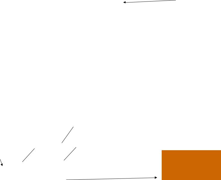
Earth’s surface heat budget

Net heat influx to a body is responsible for the heat (temperature) regime of the body.

Formulas to calculate the net heat influx are known as heat budget equations. These formulas can be drown for earth’s surface, for the atmosphere, for the earth as a planet etc.

I ' i

d BA

∆

Elementary B0

layer

	dФ *	d
	Ф
0		0

Earth’s surface

	In the soil all these fluxes suffer some variation.
	For an elementary layer the variation will be:
	dФ *Фd		dФ
			Ф * d
	Coefficient of absorption
				Heat flux
	d lnФ *	d		ln Ф	*
				Ф 0
	0	0			7

Ф Ф 0 exp *

Denoting

d

1

*

∆

* , we obtain Ф Ф 0 exp
			*

The depth the flux Ф(0) passing through decreases in “e” times.

Some amount of heat is transferred by the eddy exchange, i. e. the soil looses some heat.

QE cp K z

Evaporation of water from the soil also result in some losses of heat from the soil.

LQ'0

Under impact of all fluxes the soil temperature experiences variation, and ice (snow) melts or water freezes

L K zs Flux of latent heat

Heat flux trough the lower boundary of the layer ∆

Q	T	C * * K	T
M			m

8

The energy conservation law allows us writing the equation for a vertical soil column with the depth ∆

Income part

1 r I' i 1
		exp				*
						1
BA 1
	exp					*
					1

[C * * Km T ]

Resulting sum of these fluxes will cause:

Heat content of the layer ∆ growth up or down depending on the sign of the sum and melting snow or/and ice (if any) or freezing water.

Outgoing part

B0	1
			exp		*
					1
			cp K
				z				Z 0

L K zs Z 0

t c * *T Lmelt * t

9

m

T

1 r I ' i 1

exp

*

BA 1

exp

*

C * * K

1

1

c

K

L K

s

B

1

exp

p

0

*

z

z

1

Z 0

Z 0

c * *T L

*

t

melt

t

This equation is used to solve some particular problems. For instance, let’s take a very thin layer ∆ with no snow (ice) on it. In this case the last term is equal to 0. The term before it is very small since the layer ∆ is very thin. The term can be neglected.

* 1

* 1

0

*

1

exp

0

*

*

s

1 r I

T

'

i

BA B0

C * * Km

cp K

L K

0

z

Z 0

z

Z 0

R t	Radiation budget of the surface	10

R t

C * * Km T

cp K

L K

s

z

Z 0

z

Z 0

R(t) is a function of time and it can be presented in form of

trigonometric expansion.

Rn'

cos n t Rn'' sin n t

R t

R0

n 1

R t R0 R1 cos t tm

R value

Using two terms only,

ˆ

Time of max.

z

z

Amplitude of radiation budget diurnal variation

,t

s z,t s z x'

ˆ

R1 cos t

tm

cp K

z

T ,t T

s' c * * Km

L K

z

11