Intermediate Physics for Medicine and Biology - Russell K. Hobbie & Bradley J. Roth

6 V is the potential di erence across the resistor. If the resistance is 3 Ω, the current is i = v/R = 6/3 = 2 A. The rate of heat production in the resistor is P = vi = (6)(2) = 12 W. This could also have been calculated from P = v2/R = 36/3, or P = i2R = (4)(3). A current of 2 A means that every second 2 C of charge leave the positive terminal of the battery and flow through the resistor. When the charge arrives at the other end of the resistor, it has lost 12 J of energy to heat. The 2 C then travel through the battery back to the positive terminal, gaining 12 J from a chemical reaction within the battery.

This example has been stated as though the positive charge moves. In a metallic conductor negative charges (electrons) move from the negative terminal of the battery through the resistor to the positive terminal. In salt water and most body fluids, both positive and negative ions move. From a macroscopic point of view, we cannot tell the di erence between the transport of a charge −q from point A to point B, and the transport of a charge +q from point B to point A. Both processes make the total charge at B less positive and the total charge at A more positive by an amount q.

Two fundamental principles used in this discussion have not been stated explicitly. The first is the conservation of electric charge: all charge that leaves the battery passes through the resistor. The second is the conservation of energy: a charge that starts at some point in the circuit and comes back to its starting point has neither lost nor gained energy. (The energy gained by a charge in the battery is equal to the energy lost by it in passing through the resistor.) These principles become less obvious and more useful in a circuit that is more complicated than the one considered above. They are known as

Kirchho ’s laws.

In a more complicated circuit, Kirchho ’s first law (conservation of charge) takes the following form. Any junction where the current can flow in di erent paths is called a node. The algebraic sum of all the currents into a node is zero. (By algebraic sum we mean that currents into the node are positive, while currents leaving the node are negative, or vice versa.) This ensures that no charge will accumulate at the node.11

As an example of Kirchho ’s first law, consider the node in Fig. 6.22. Conservation of charge requires that 2 + 3 + i = 0 or i = −5 A. (In this case positive currents flow into the node; the negative current means that 5 A is flowing out of the node as current i.)

11More generally, the node could represent a conductor, such as the plate of a capacitor, on which charge can accumulate. In that case the charge Q changes with time:

dQ = (all currents into the node). dt

6.9 The Application of Ohm’s Law to Simple Circuits

147

FIGURE 6.22. Conservation of charge means that current i is −5 A.

FIGURE 6.23. A more complicated circuit, sometimes called a voltage divider.

Kirchho ’s second law was used implicitly in the example above to say that the voltage across the resistor is 6 V. In general, Kirchho ’s second law says that if one goes around any closed path in a complicated circuit, the total voltage change is zero.

Kirchho ’s laws can be applied to show that the total resistance of a set of resistors in series is

R = R1 + R2 + R3 + · · · .

This follows from the definition of resistance, the fact that the same current flows in each resistor, and the total potential di erence across the set of resistors is the sum of the potential di erence across each one. Kirchho ’s laws can also be used to show that for a collection of resistors in parallel, the total resistance is given by

1	=	1		1		1
				+		+		+ · · · ,
R		R1			R2		R3

(see Problem 23).

Consider a more complicated example in which two resistors are connected across a battery. The battery voltage is v, and the resistances are R1 and R2, as shown in Fig. 6.23. If no current flows out lead A, then conservation of charge requires that the same current i flows in each resistor. The sum of the voltages v1 and v2 is v. Therefore, i = v1/R1 = v2/R2 and v = v1 + v2 = iR1 + iR2 = i(R1 + R2). The voltage across R2 is iR2 or

	This statement is quite similar to the continuity equation of Sec.			R2
	4.1.
		v2	= R1 + R2 v.			(6.31)

148 6. Impulses in Nerve and Muscle Cells

v

E

+		Ð		Ð		+
+		Ð		Ð		+
Outside +		Ð	Inside	Ð		+	Outside
+		Ð		Ð		+
+		Ð		Ð		+

FIGURE 6.24. The potential, electric field, and charge at different points on the diameter of a resting nerve cell. Portions of the cell membrane on opposite sides of the cell are shown. Outside the cell on the left the potential and electric field are zero. As one moves to the right into the cell, the electric field in the membrane causes the potential to decrease to −70 mV. Within the cell the field is zero and the potential is constant. Moving out through the right-hand wall the potential rises to zero because of the electric field within the membrane.

6.10Charge Distribution in the Resting Nerve Cell

The axon consists of an ionic intracellular fluid and an ionic extracellular fluid, separated by a membrane. The intracellular and extracellular media are electrical conductors. When the cell is in equilibrium there is no current and no electric field in these regions. There will be a field and currents when an impulse is traveling along the axon.

Because the electric field in the resting cell is zero, there is no net charge in the fluid. Positive ions are neutralized by negative ions everywhere except at the membrane. A layer of charge on each surface generates an electric field within the membrane and a potential di erence across it.

Measurements with a microelectrode show that the potential within the cell is about 70 mV less than outside. If the potential outside is taken to be zero, then the interior resting potential is −70 mV. Figure 6.24 shows a slice across the cell, showing the membrane on opposite sides of the cell and the charges and electric field. If the potential drops 70 mV as one enters the cell on the left, if the membrane thickness is 6 nm, and if the electric field within the membrane is assumed to be constant, then

E = −dv = −−70 × 10−3 V = 1.17 × 107 V m−1. dx 6 × 10−9 m

(6.32) This is how the value of E was determined for use on p. 141.

Except for the layers of charge on the inside and outside of the membrane, which are shown in Fig. 6.24 and which give rise to the electric field and potential di erence, the extracellular and intracellular fluids are electrically neutral. However, the ion concentrations are quite di erent in each (Fig. 6.3). There is an excess of sodium ions outside and an excess of potassium ions inside.

It is possible to see which concentrations (if any) are consistent with the hypothesis that the ions can pass freely through the membrane. If a species is in equilibrium, the concentration ratio ci/co across the membrane is given by a Boltzmann factor or the Nernst equation (see Chapter 3). The potential energy of the ion is zev, where z is the valence of the ion, e the electronic charge (1.6 × 10−19 C), and v the potential in volts. Using subscripts i and o to represent inside and outside the cell, we have

	ci	=	e−zevi /kB T	= e−ze(vi −vo )/kB T .	(6.33)
	co		e−zevo /kB T

Here kB is Boltzmann’s constant, 1.38 × 10−23 J K−1. For a situation in which T = 310 K and vi − vo = −70×10−3 V, ci/co is 13.7 for univalent positive ions and 1/13.7 = 0.073 for negative ions. The ratios in Fig. 6.3 are 0.103 for sodium, 30 for potassium, and 0.071 for chloride. The chloride concentration ratio is consistent with equilibrium, while the sodium concentration ratio is much too small (too few sodium ions inside) and the potassium concentration ratio is too large (too many potassium ions inside).

A potential of −90 mV would bring the potassium concentration ratio into equilibrium, but then chloride would not be in equilibrium and sodium would be even farther from equilibrium. In fact, tracer studies show that potassium leaks out slowly and sodium leaks in slowly. The resting membrane is not completely impermeable to these ions [Hodgkin (1964, Chapter 6); La¨uger (1991)]. To maintain the ion concentrations a membrane protein called the sodium-potassium pump uses metabolic energy to pump potassium into the cell and sodium out. The usual ratio of sodium to potassium ions in this active transport is 3 sodium to 2 potassium ions [Patton et al. (1989, Vol. 1, p. 27)].

The intracellular and extracellular fluids can be modeled as two conductors separated by a fairly good insulator. The conductors have a capacitance between them. We can estimate this capacitance in two ways. We can either regard the membrane as a plane insulator sandwiched between plane conducting plates (as if the membrane had been laid out flat as in Fig. 6.25), or we can treat it as a dielectric between concentric cylindrical conductors. The text will use the first approximation, while the second will be left to a problem. Suppose that two parallel plates have area S and charge ±Q, respectively, then the charge density on each is σ = ±Q/S. Equation 6.11 gives the electric field without a dielectric between the conductors: Eext = σ/ 0 = Q/ 0S.

FIGURE 6.25. A portion of a cell membrane of length L, in its original configuration and laid out flat. The membrane thickness is b and the radius of the axon is a. The plane approximation is used to calculate both the capacitance and resistance of the membrane.

With the dielectric of dielectric constant κ, the field is reduced to E = Eext/κ = σ/κ 0 = Q/κ 0S, as was seen in Eq. 6.20. The magnitude of the potential di erence is E times the plate separation b: v = Eb = Qb/κ 0S. The capacitance is C = Q/v:

C =	Qκ 0S	=	κ 0S	.	(6.34)
	Qb
			b

The charge density on the surface of the membrane is obtained from σ = Q/S = Cv/S = κ 0v/b.

Measurements of the dielectric constant κ for axon membrane show it to be about 7. Using values of −70 mV for v and 6 nm for b, the capacitance per unit area of membrane can be calculated, as can σ:

	C	=	(7)(8.85 × 10−12)	= 0.01 F m−2 = 1 µF cm−2,
	S		6 × 10−9

σ = (0.01)(70 × 10−3) = 7 × 10−4 C m−2. (6.35)

This value for the surface charge density is larger by a factor of 7 than that calculated in Sec. 6.3. The reduction of the electric field by polarization of the dielectric has been taken into account in the present calculation. A larger external charge is required to give the same field within the dielectric.

The value of b for myelinated fibers is much greater, typically 2000 nm instead of 6 nm. This reduces the capacitance per unit area by a factor of 300.

6.11 The Cable Model for an Axon

We now consider the rather complicated flow of charge in the interior of an axon, through the membrane, and

6.11 The Cable Model for an Axon

149

INTERIOR

CONDUCTING FLUID

C

+

+ + +

+ +

+

Q

+

−

+

Rm

+C

i m

R

v

i m

v

m

−

−

− − − − − − −

−Q

EXTERIOR

CONDUCTING FLUID

(a)

(b)

(c)

FIGURE 6.26. Leakage currents through the membrane. (a) The flow of positive and negative ions. (b) The membrane capacitance is represented by the parallel plates and the leakage resistance by a single resistor. (c) The capacitance and resistance are usually drawn like this.

in the conducting medium outside the cell during departures from rest. We will model the axon by electric conductors that obey Ohm’s law inside and outside the cell and a membrane that has capacitance and also conducts current. We will apply Kirchho ’s laws—conservation of energy and charge—to a small segment of the axon. The result will be a di erential equation that is independent of any particular model for the cell membrane. This is called the cable model for an axon. We will then apply the cable model in two cases. The first case is when the voltage change does not alter the properties of the membrane. The second case is a voltage change that changes the ionic permeability of the membrane, thereby generating a nerve impulse.

Consider the small segment of membrane shown in Fig. 6.26(a). For the moment we ignore the resting potential on the membrane. We will see later that accounting for the resting potential requires only a small change to the model. The upper capacitor plate, corresponding to the inside of the membrane, carries a charge Q. The lower capacitor plate (the outside of the membrane) has charge −Q. The charge on the membrane is related to the potential di erence across the membrane by the membrane capacitance Cm: Q = Cmv. Figure 6.26(a) shows positive ions on the inside and negative ions on the outside of the membrane. (In a resting nerve cell, there is negative charge on the inside of the membrane, Q is negative, −Q is positive, and v < 0.)

If the resistance between the plates of a capacitor is infinite, no current flows, and the charge on the capacitor plates remains constant. However, a membrane is not a perfect insulator; if it were, there would be no nerve conduction. Some current flows through the membrane. We call this current im and define outward current to be positive, as in Fig. 6.26(b).

Imagine for now that there is no current along the axon. In that case im discharges the membrane capacitance, and the charge and potential di erence fall to zero as charge flows through the resistor. When im is positive, Q

150 6. Impulses in Nerve and Muscle Cells

and v decrease with time:
−im =	dQ	= Cm	dv		(6.36)
				.
	dt		dt

Let us explore the behavior of this isolated segment of axon a bit further. For now we think of the total leakage current as being through a single e ective resistance Rm. This is shown in Fig. 6.26(b). It is customary to draw the resistance separately, as in Fig. 6.26(c). The current is then im = v/Rm and Cm(dv/dt) = −im = −v/Rm,

dv	1
	= −		v.	(6.37)
dt		RmCm

This is the familiar equation for exponential decay of the voltage (see Chapter 2). If the initial voltage at t = 0 is v0, the solution is

v(t) = v0e−t/τ ,	(6.38)
where the time constant τ is given by
τ = RmCm.	(6.39)

Referring to Fig. 6.25, we saw that if we have a section of membrane of area S and thickness b the capacitance is given by Eq. 6.34. For a conductor of the same dimensions we saw [Eq. 6.27] that the resistance is Rm = ρmb/S, so

the time constant is
τ = RmCm =	ρmb		κ 0S	= κ 0ρm.	(6.40)
	S b

We have the remarkable result that the time constant is independent of both the area and thickness of the membrane. Doubling the area S doubles the amount of charge that must leak o , but it also doubles the membrane current. Doubling b doubles the resistance, but it also makes the membrane capacitance half as large. In each case the factors S and b cancel in the expression for the time constant.

If a very thin lipid membrane is produced artificially, it is found to have a very high resistivity—about 1013 Ω m [Scott (1975, p. 493)]. Certain proteins added to the lipid material reduce the resistivity by several orders of magnitude. For natural nerve membrane the resistivity is about

ρm = 1.6 × 107 Ω m.

(6.41)

This is the e ective resistivity for resting membrane, taking into account all of the ion currents. If ρm had this constant value the time constant would be τ = κ 0ρm = (7)(8.85 × 10−12)(1.6 × 107) = 1 × 10−3 s. (Actually, the resistivity changes drastically as the potential across the membrane changes during the propagation of a nerve impulse.) Since we observe a potential di erence across the membrane, there must be a mechanism for renewing the charge on the membrane surface.

The resistance and capacitance of the portion of the axon membrane in Fig. 6.25 can be written in terms of

the axon radius a and the length L of the segment by noting that S = 2πaL. Then one has

Cm =	κ 02πaL	,	Rm =	ρmb	.
	b
				2πaL

It is convenient to recall that v = iR can be written as i = Gv and introduce the conductance of the membrane segment

Gm =	2πaL	.	(6.42)
	ρmb

Both the capacitance and the conductance are proportional to the area of the segment S. It is also convenient to introduce the lowercase symbols cm and gm to stand for the membrane capacitance and membrane conductance

	per unit area:		Cm		κ 0
	cm =			=				,			(6.43)
			S				b
	gm =	Gm	=	1			=		σm	.	(6.44)
		S		ρmb					b

(Remember that σm = 1/ρm is the electrical conductivity, the reciprocal of the resistivity. It is not the charge per unit area. σ is frequently used for both quantities in the literature.)

Both cm and gm depend on the membrane thickness as well as the dielectric constant and resistivity of the membrane. The units of cm and gm are, respectively, F m−2 and S m−2. Be careful: many sources give them per square centimeter instead of per square meter.

We can rewrite Eq. 6.36 in terms of the current density, jm, which is proportional to the capacitance per unit

area, cm:
−jm = cm	dv		(6.45)
		.
	dt

Table 6.1 shows typical values for these quantities and some to be discussed later for an unmyelinated axon.12 These values should not be associated with a particular species. Parameters such as the resistance and capacitance per unit length of the axon are measured directly. Others, such as ρm, require an estimate of membrane thickness and are less well known

Now let us consider current that flows inside and outside the axon. Assume that the currents inside are longitudinal, that is, parallel to the axis of the axon. A discussion of departures from this assumption is found in Scott

12Some insight into the magnitude of the charge on the membrane can be obtained from these numbers. The excess charge on the surface of the membrane is 7 × 10−4 C m−2 for the unmyelinated fiber. This corresponds to 4.4 × 1015 ions per square meter, if each ion has a charge of 1.6 × 10−19 C. Each atom or ion in contact with the membrane surface occupies an area of about 10−20 m2; thus there are about 1020 atoms or ions in contact with a square meter of membrane surface. These may be neutral or positively or negatively charged. If charged, most are neutralized by the presence of a neighbor of opposite charge. The excess charge density that is required can be obtained if 4.4 × 1015/1020 or roughly one out of every 20, 000 of the atoms in contact with the surface is ionized and not neutralized.

TABLE 6.1. Properties of a typical unmyelinated nerve.

a	Axon radius	5 × 10−6 m
b	Membrane thickness	6 × 10−9 m
ρi	Resistivity of	0.5 Ω m
	axoplasm	6.4 × 109 Ω m−1
ri = ρi/πa2	Resistance per unit
	length inside axon
κ	Dielectric constant of	7a
	membrane	1.6 × 107Ω m
ρm	Resistivity of
	membrane	112 × 106 Ω m
κρm
cm = κ 0/b	Membrane	10−2 F m−2
	capacitance per
	unit area	3 × 10−7 F m−1
2πκ 0a/b	Membrane
	capacitance per
	unit length of axon
gm = 1/ρmb	Conductance per unit	10 S m−2
.1/gm	area of membrane
	Reciprocal of	0.1 Ω m2
	conductance per unit
	area	3.2 × 10−4 S m−1
2πa/ρmb	Membrane
	conductance per
	unit length of axon	−70 mV
vr	Resting potential
	inside axon	1.2 × 107 V m−1
E = vr /b	Electric field
	in membrane	7 × 10−4 C m−2
κ 0vr /b	Charge per unit area
	on membrane surface	4.4 × 1015 m−2
	Net number of
	univalent ions per
	unit area	6.6 × 107 m−1
	Net number of
	univalent ions per
	unit length

aSee Sec. 6.17 for a discussion of the dielectric constant.

(1975, p. 492). With this assumption, the interior fluid can be regarded as a resistance of length L and radius a as shown in Fig. 6.27. The resistance of such a segment is Ri = ρiL/S = ρiL/πa2. It is convenient to work with the resistance per unit length, ri:

Ri		=		ρi			1
ri =						=		.	(6.46)
	L		πa		2		2
							πa σi

The question of resistance of the extracellular fluid for currents outside the axon is more complicated. If the extracellular fluid were infinite in extent, the longitudinal resistance outside the cell would be very small (see Chapter 7). On the other hand, in a nerve or a muscle the axons or muscle cells are packed closely together, there is not very much extracellular fluid, and the external resistance

6.11 The Cable Model for an Axon

151

FIGURE 6.27. Axoplasm of length L and radius a can be treated like a simple resistor.

i i (x)

i i (x + dx)

a

xx + dx

im

FIGURE 6.28. The membrane surrounding a small portion of an axon is shown, along with the longitudinal currents in and out of the segment.

per unit length can be significant. There are some important e ects that occur because of this. We will discuss them in Chapter 7.

Now we can consider the e ect of both membrane and longitudinal currents. Figure 6.28 shows a small region of the axon between x and x + dx and the surrounding membrane. Current ii flows longitudinally along the axon on the inside. The current through the membrane is im. The potential di erence across the membrane is v = vi − vo. In this section no attempt will be made to relate im or jm to v. Charge Q resides on the inside surface of the membrane and can be either negative or positive. An equal and opposite charge −Q resides on the outer surface of the membrane.

Because the capacitance can charge or discharge, Kirchho ’s law (conservation of charge) does not say that the sum of the currents is zero. Rather, it says that the net current into the volume of axoplasm between x and x + dx changes the charge on the interior surface of the membrane:

i	(x)	i (x + dx)	i		=	dQ		= C	d(vi − vo)	. (6.47a)
							dt		m dt
i		− i	−	m

When ii(x) = ii(x + dx) this gives Eq. 6.36. The membrane current im represents an average value for the segment of membrane between x and x + dx. It is also a function of x.

152 6. Impulses in Nerve and Muscle Cells

It is necessary to use partial derivatives because the current and voltage depend on both x and t as an impulse travels down the nerve. As dx → 0

ii(x + dx) − ii(x)	→	∂ii	.
dx
		∂x

This can be evaluated using the expression for Ohm’s law in the axoplasm, Eq. 6.48:

∂ii	= −	1 ∂2vi				(6.50)
					.
∂x		ri		∂x2

When this is inserted in Eq. 6.49 the result is

c		∂(vi − vo)	=	j		+	1		∂2vi	.	(6.51)
	m	∂t		−	m		2πa ri ∂x2

FIGURE 6.29. A hypothetical plot of vi(x) and the longitudinal current ii associated with it.

We can define dii = ii(x + dx) − ii(x) as the increase in ii along segment dx. Then we can rewrite Eq. 6.47a as

dv	+ im.
−dii = Cm dt		(6.47b)

This is an important equation. It says that when the current flowing inside the axon decreases in a small distance dx, part of the current charges the capacitance of that segment of membrane, and the rest flows through the membrane.

Consider a small segment of axoplasm of length dx. The intracellular voltage at the left end is vi(x); at the right end it is vi(x + dx). The current along the segment is the voltage di erence between the ends divided by the resistance of the segment. The resistance is Ri = ri dx. Therefore, the current is

i	(x) =	vi(x) − vi(x + dx)	=		1		dvi	.	(6.48)
		ri dx
i				−ri dx

The voltage must change along the axon for a current to flow within it. The minus sign in Eq. 6.48 shows that a current flowing from left to right (in the +x direction) requires a voltage that decreases from left to right, and vice versa.

Figure 6.29 shows a hypothetical plot of vi(x) and the current which would accompany it. Notice that the current is flowing from the region of higher voltage to lower voltage–towards both ends from the region between x1 and x2. In that region either the charge on the membrane is changing or current is flowing through the membrane.

Consider again the cylindrical geometry shown in Fig. 6.28. The surface area of this portion of membrane is 2πa dx. Dividing each term of Eq. 6.47a by the area and remembering the definitions of jm and cm we obtain

c		∂v	=	j		+	1		ii(x) − ii(x + dx)		. (6.49)
	m ∂t						2πa
				−	m				dx

In many cases the extracellular potential is small. In that case the voltage across the membrane, v, is approximately the same as the intracellular voltage, vi, so we can rewrite Eq. 6.51 as

	∂v	= −jm +	1 ∂2v				(6.52)
cm						.
	∂t		2πa ri		∂x2

This rather formidable looking equation is called the cable equation or Telegrapher’s equation. It has the form of Fick’s second law of di usion, Eq. 4.26, with the addition of the jm term.

It is worth recalling the origin of each term and verifying that the units are consistent. The term on the left is the rate at which the membrane capacitance is gaining charge per unit area. Therefore, all terms in the equation have the units of current per unit area. The first term on the right is the current per unit area through the membrane in the direction that discharges the membrane capacitance. The second term on the right gives the buildup of charge on this area of the membrane because of di erences in current along the axon. If v(x) were constant, there would be no current along the inside of the axon. If function v(x) had constant slope, the current along the inside of the axon would be the same everywhere and there would be no charge buildup on the membrane. It is only because v(x) changes slope that ii is di erent at two neighboring points in the axon and charge can collect on the membrane.

Now, for the units. Since i = C(dv/dt), the units of cm∂v/∂t are current per unit area. The jm term is by definition current per unit area. Since ri has the units of Ω m−1, the term 2πari, has the units of Ω. When this is combined with ∂2v/∂x2, which has units V m−2, the result is A m−2 as required.

This is a very general equation stating Kirchho ’s laws for a segment of the axon. The only assumptions are that the currents depend only on time and position along the axon and that voltage changes on the outside of the axon can be neglected. Particular models for nerve conduction use di erent relations between jm and v(x, t).

6.12 Electrotonus or Passive Spread

153

6.12 Electrotonus or Passive Spread

The simplest membrane model is one that obeys Ohm’s law. This approximation is valid if the voltage changes are small enough so that the membrane conductance does not change, or if something has been done to inactivate the normal changes of membrane conductance with voltage. It is also useful for myelinated nerves between the nodes of Ranvier. This is called electrotonus or passive spread.

In its quiescent state, the voltage all along the inside of the axon has the constant resting value vr . Both ∂v/∂t and ∂2v/∂x2 are zero. Equation 6.52 can be satisfied only if jm = 0. Although jm is zero, it may be made up of several leakage components. In this section we simply assume

that jm is proportional to v − vr :
jm = gm(v − vr ).	(6.53)

This simple model does predict that jm = 0 when v = vr . It also predicts that the current will be positive (outward) if v > vr and negative (inward) if v < vr . It does not explain the propagation of an all-or-nothing nerve impulse. The conductance per unit area, gm, is assumed to be independent of v and of the past history of the membrane. This is a good assumption only for very small voltage changes. With this assumption, Eq. 6.52 becomes

	∂v	= −gm(v − vr ) +	1 ∂2v				(6.54)
cm						.
	∂t		2πa ri		∂x2

This equation is usually written in a slightly di erent form by dividing through by gm:

1 ∂2v			− v −	cm ∂v			= −vr .
2πa rigm		∂x2		gm		∂t

It is also customary to make the assignments

λ2 =	1	,
	2πa rigm

τ= cm , gm

so that the equation becomes
λ2	∂2v	− v − τ	∂v	= −vr .	(6.55)
	∂x2		∂t

In terms of the primary axon parameters, the parameters in Eq. 6.55 are

λ2 =	abρm	,	(6.56)
	2ρi
τ = κ 0ρm.			(6.57)

The time constant was seen before in Eq. 6.40. Equation 6.55 has a steady-state solution v = vr . If a new variable v = v − vr is used, it becomes the homogeneous version of the same equation with a steady-state solution v = 0. This homogeneous equation is known as the

FIGURE 6.30. The voltage distribution along an axon in electrotonus when the membrane capacitance is charged and the voltage is not changing with time.

telegrapher’s equation: it was once familiar to physicists and electrical engineers as the equation for a long cable, such as a submarine cable, with capacitance and leakage resistance but negligible inductance [Je reys and Je reys (1956, p. 602)].

For nerve conduction, the inhomogeneous equation with various exciting terms corresponding to physiological stimuli was discussed by Davis and Lorente de N´o (1947) and by Hodgkin and Rushton (1946). Their work is summarized by Plonsey (1969, p. 127).

Before considering general solutions to Eq. 6.55, consider some special cases. If cm = 0, so that τ = 0, or if enough time has elapsed so that the voltage is not changing with time and ∂v/∂t = 0, the equation reduces to

λ2 ∂2v − v = −vr . ∂x2

You can verify by substitution that this has a solution

$ v0e−x/λ,		x > 0	(6.58)
v − vr =	v0ex/λ,	x < 0.

If the voltage is held at a constant value v = vr + v0 at some point on the axon, the voltage will decay exponentially to vr in both directions from that point. This is shown in Fig. 6.30.

Next, suppose that v(x, t) does not depend on x, so that there is no longitudinal current in the axon and ∂2v/∂x2 = 0. This can be accomplished experimentally by threading a wire axially along the axon, if the axon is fat enough. The equation reduces to

∂v

τ ∂t + v = vr .

This is the familiar equation for exponential decay. If v were held at v0 +vr and then the constraint were removed at t = 0, the voltage would decay exponentially back to

vr

v − vr = v0e−t/τ .

154 6. Impulses in Nerve and Muscle Cells

	1.0				(a)	1.0
	0.8					0.8
0					0
r)/v	0.6	t = ∞			r)/v	0.6
(v(x,t)-v	0.4	t = τ			(v(x,t)-v	0.4
						0.2
	0.2
		t = τ/4
	0.0					0.0
			2
	0	1		3	4
			x/λ

				(b)
	x = 0
		x = λ
			x = 2λ
0	1	2	3	4
		t/τ

FIGURE 6.31. Some representative solutions to the problem of electrotonus after the application of a constant current at x = 0. (a) The voltage along the axon at di erent times (b) Voltage at a fixed point on the axon as a function of time.

This represents the discharge of the membrane capacitance through the membrane resistance.

The behavior of v(x, t) − vr at various times after an excitation is applied is shown in Fig. 6.31. The excitation is a constant current injected at x = 0 for all time t > 0. After a long time, the curve is identical to that in Fig. 6.30, as the membrane capacitance has fully charged. Only the membrane leakage current attenuates the signal. At earlier times the solution is not precisely exponential; the analytic solution involves error functions (Problem 34). The change of voltage with time at fixed positions along the cable is also shown. Both the finite propagation time and the attenuation of the signal are evident.

6.13The Hodgkin–Huxley Model for Membrane Current

If the voltage at some point on the axon changes by a few millivolts from the resting value, the voltage at other points on the axon is described by electrotonus. However, if the inside voltage rises from the resting value by 20 mV or more, a completely di erent e ect takes place. The potential rises rapidly to a positive value, then falls to about −80 mV, and finally returns to the resting value (Fig. 6.1). This behavior is attributable to a very nonlinear dependence of membrane current on transmembrane voltage.

Considerable work was done on nerve conduction in the late 1940s, culminating in a model that relates the propagation of the action potential to the changes in membrane permeability that accompany a change in voltage. The model [Hodgkin and Huxley (1952)] does not explain why the membrane permeability changes; it relates the shape and conduction speed of the impulse to the observed changes in membrane permeability. Nor does it explain all the changes in current. (For example, the potassium current does fall eventually, and there are some properties of the sodium current that are not adequately described.) Nonetheless, the work was a triumph that led to the Nobel Prize for Alan Hodgkin and Andrew Huxley.

FIGURE 6.32. Apparatus for voltage-clamp measurements.

Most of the experiments that led to the Hodgkin– Huxley model were carried out using the giant axon of the squid. This is a single cell several centimeters long and up to 1 mm in diameter that can be dissected from the squid. The removal of axoplasm from the preparation and its replacement by electrolytes has shown that the critical phenomena all take place in the membrane. The important results are reviewed in many places [Katz (1966, Chapters 5 and 6); Plonsey (1969, p. 127); Plonsey and Barr (1988, Ch. 4); Scott (1975, pp. 495–507)].

6.13.1Voltage Clamp Experiments

Voltage-clamp experiments were particularly illuminating. Two long wire electrodes were inserted in the axon and connected to the apparatus shown in Fig. 6.32. The resistance of the wires was so low that the potential at all points along the axon was the same at any instant of time. The potential depended only on time, and not on position. This is called a space-clamped experiment. One electrode, paired with an electrode in the surrounding medium, measured the voltage di erence across the membrane. The other electrode was used to inject or remove whatever current was necessary to keep this voltage di erence constant. Measurement of this current allowed calculation of the membrane conductance. This technique is called voltage clamping. The experiment described here was both voltageand space-clamped.

When the membrane potential was raised abruptly from the resting value to a new value and held there, the resulting current was found to have three components:

1.A current, lasting a few microseconds, that changed the surface charge on the membrane.

2.A current flowing inward which lasted for 1 or 2 ms. Various experiments, such as replacing the sodium ions in the extracellular fluid with some other monovalent ion, showed that this was due to the inward flow of sodium ions. (Had the potential not been voltage-clamped by the electronic apparatus, this inrush of positive charge would have raised the potential still further.)

6.13 The Hodgkin–Huxley Model for Membrane Current

155

3. An outward current that rose in about 4 ms and			inside
remained steady for as long as the potential was	+		jNa
clamped at this value. Tracer studies showed that
this current was due to potassium ions. (Over a time	v		gNa
scale of several tens of milliseconds, the potassium
			+
current, like the sodium current, does fall back to				= 50 mV
zero.)			vNa
	Ð		Ð

The first current is the cm(∂v/∂t) term of Eq. 6.52; the second and third currents together constitute jm. Because of the clamping wires, the ∂2v/∂x2 term is zero.

The next step is to develop a model that describes the major ionic constituents of the current. The sodium and potassium contributions to the current will be considered separately; all other contributions will be combined in a “leakage” term:

outside

(a)

jm

gK

gNa

gL

jm = jN a + jK + jL.

(6.59)

The leakage includes charge movement due to chloride ions and any other ions that can pass through the membrane.

Consider movement of sodium through the membrane. Similar considerations apply to potassium. The concentrations of sodium inside and out are [Nai] and [Nao]. It will be seen later that the total number of ions moving through the membrane during a nerve pulse in a squid giant axon is too small to change the concentrations significantly. Therefore, the concentrations are fixed.

There would be no movement of sodium ions through the membrane, regardless of how permeable it is, when the concentrations and potential are related by the Boltzmann factor or Nernst equation (Eq. 6.33) with v = vi − vo:

[Nai] = e−ev/kB T .

[Nao]

For given concentrations, the sodium Nernst potential is

vN a =	kB T	ln		[Nao]	.
	e			[Nai]

equilibrium or

(6.60)

The sodium Nernst potential is usually about 50 mV. If v = vN a there is no current of sodium ions, regardless of the membrane permeability to sodium. If v is greater than vN a (more positive), jN a flows outward. If v < vN a, the sodium current is inward. These currents can be described by

jN a = gN a(v − vN a).

(6.61)

The coe cient gN a is the sodium conductance per unit area. It is not constant but depends on the value of v and, in fact, on the past history of v. Defining the conductance this way makes the functional form of gN a less complex; in particular, it does not have to change sign as v moves through vN a and the sodium current reverses direction.

This equation can be multiplied by the membrane area to give a current–voltage relationship. Many authors draw a circuit diagram to represent the current flow

		v					v				vL
				K					Na

(b)

FIGURE 6.33. Equivalent circuits for the membrane current.

(a) The sodium current–voltage relationship of Eq. 6.61 is the same as that for a variable resistance in series with a battery at the sodium Nernst potential. (b) The total membrane current can be modeled with three such equivalent circuits. See the discussion of the sign of the potassium and leakage Nernst potentials in the text.

through the membrane and along the axon. The sodium voltage–current relationship can be represented by a variable resistance corresponding to gN a in series with a battery at the sodium Nernst potential, as shown in Fig. 6.33(a).

An expression similar to Eq. 6.61 can be written for the potassium current density:

jK = gK (v − vK ).

(6.62)

The potassium Nernst potential is negative—about −77 mV—so the polarity of the potassium battery in Fig. 6.33(b) has been reversed. The leakage term will be considered later.

To summarize: v is the instantaneous voltage across the membrane. Both vK and vN a are constants depending on the relative ion concentrations inside and outside the cell and the temperature. The conductances per unit area depend on both the present value of v and its past history.

We can now describe the results of the voltage clamp experiments. The voltage in each experiment was changed from the resting value by an amount ∆v. Therefore, v −vN a and v −vK had constant values after the change, and the changes in current density mirrored the changes in conductivity. Typical results for ∆v = 25 mV and T = 6 ◦C are shown in Figs. 6.34 and 6.35. [The method of distinguishing sodium from potassium current is described in the original papers, or in Hille (2001, p. 39).]

156 6. Impulses in Nerve and Muscle Cells

	80
					gK
	60
)
Ð2
m
ΩÐ1	40
(
Na
g				v = -40 mV
or
				vr = -65 mV
K
g				v - vr = +25 mV
	20
					gNa
	0	2	4	6	8	10
	0

t (ms)

	200
				v = -20 mV
	150
)				v = -30 mV
Ð2
m	100
Ð1
(Ω
K
g					v - -40 mV
	50
				v = -50 mV
	0
	0	2	4	6	8	10

t (ms)

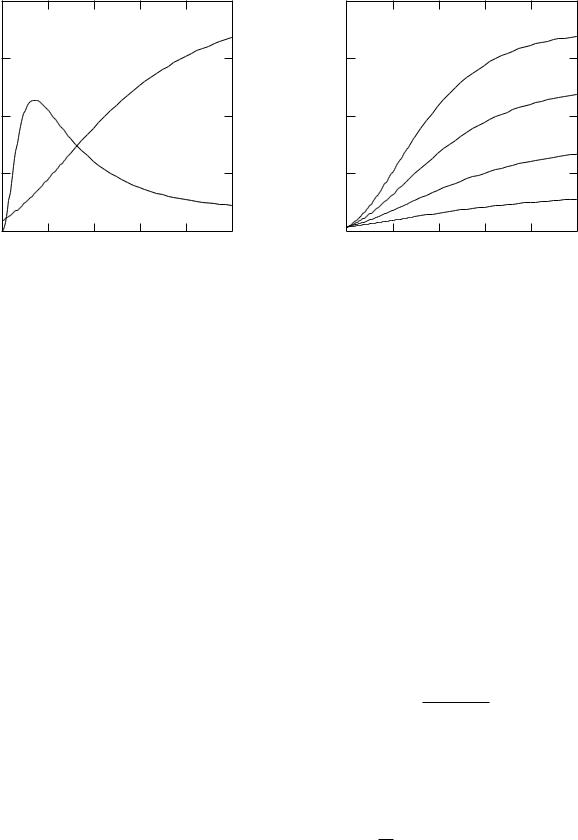
FIGURE 6.34. The behavior of the sodium and potassium conductivities with time in a voltage-clamp experiment. At t = 0 the voltage was raised by 25 mV from the resting potential. The values are calculated from Eqs. 6.64–6.71 and are representative of the experimental data.

For a voltage clamp experiment the current and conductance have the same time variation. The sodium conductance rises from zero and then falls, while the potassium conductance rises more slowly from a small initial resting value. (The potassium current before the voltage clamp was applied was small, because the resting potential was close to the potassium Nernst potential.) Measurements for longer times show that the potassium conductivity rises to a constant value. Measurements for much longer times show that the potassium current falls after tens of milliseconds. For other values of ∆v the conductance changes are di erent.

6.13.2Potassium Conductance

Hodgkin and Huxley wanted a way to describe their extensive voltage-clamp data, similar to that in Figs. 6.34 and Fig. 6.35, with a small number of parameters. If we ignore the small nonzero value of the conductance before the clamp is applied, the potassium conductance curve of

Fig. 6.34 is reminiscent of exponential behavior, such as gK (v, t) = gK (v)(1 −e−t/τ (v)), with both gK (v) and τ (v) depending on the value of the voltage. A simple exponential is not a good fit. Figure 6.36 shows why. The curve (1−e−t/τ ) starts with a linear portion and is then concave downward. The potassium conductance in Figs. 6.34 and 6.35 is initially concave upward. The curve (1−e−t/τ )4 in Fig. 6.36 more nearly has the shape of the conductance data. This suggests that we try to describe the conductance by

N

gK (v, t) = gK∞ n∞(v)(1 − e−t/τ (v)) . (6.63)

FIGURE 6.35. The behavior of the potassium conductance for di erent values of the clamping voltage. These are representative curves calculated from Eqs. 6.64–6.66.

In this expression, gK∞ is the largest possible conductance per unit area. The value of n∞(v) varies between 0 and 1 and determines the asymptotic value of the conductance change for a particular value of the voltage step. Hodgkin and Huxley found a good fit to their data with N = 4. If the initial value of the conductance were zero, our empirical fit to the potassium conductance data would be

g	K	(v, t) = g	K∞	n4	(v, t),	(6.64a)
n(v, t) = n∞(v)(1 − e−t/τ (v)).						(6.64b)

But the initial potassium conductance was not zero. How should this be handled? Hodgkin and Huxley assumed that n is a measure of some fundamental property of the potassium channels, and that the conductance is always described by Eq. 6.64a. When the clamp voltage changes, the subsequent change of n is described by an exponential decay with the appropriate values of n∞(v) and τ (v). If the initial value of n is n0, the expression for n(v, t) after the voltage clamp change is

n(v, t) = n	(v) 1		n∞(v) − n0	e−t/τ (v) . (6.64c)
∞		−	n∞(v)

The function n is a solution to the di erential equation

dn	= −	n	+	n∞			(6.65a)
dt		τ			τ	.

Hodgkin and Huxley wrote this instead in the form

dn	= αn(1 − n) − βnn.	(6.65b)
dt

The subscript n on αn and βn distinguishes them from similar parameters for the sodium conductance.