Intermediate Physics for Medicine and Biology - Russell K. Hobbie & Bradley J. Roth

	8
	7
	6
	5
t	4
y=e
	3
	2
	1
	0
	-2	-1	0	1	2
			t
FIGURE 2.2. A graph of the exponential function y = et.

look up the exponential function of this amount in a table or evaluate it with a computer or calculator. The number e is approximately equal to 2.71828 . . . and is called the “base of the natural logarithms.” Like π (3.14159 . . . ) e has a long history [Maor (1994)].

The exponential function is plotted in Fig. 2.2. (The meaning of negative values of t will be considered in the next section.) This function increases more and more rapidly as t increases. This is expected, since the rate of growth is always proportional to the present amount. This is also reflected in the following property of the exponential function:

d	ebt	= bebt.	(2.5)
dt

This means that the function y = y0ebx has the property that

	dy	= by.	(2.6)
	dt

Any constant multiple of the exponential function ebt has the property that its rate of growth is b times the function itself. Whenever we see the exponential function, we know that it satisfies Eq. 2.6. Equation 2.6 is an example of a di erential equation. If you learn how to solve only one di erential equation, let it be Eq. 2.6. Whenever we have a problem in which the growth rate of something is proportional to the present amount, we can expect to have an exponential solution. Notice that for time intervals t that are not too large, Eq. 2.6 implies that ∆y = (b∆t)y. This again says that the increase in y is proportional to y itself.

The independent variable in this discussion has been t. It can represent time, in which case b is the fractional

2.2 Exponential Decay

33

growth rate per unit time; distance, in which case b is the fractional growth per unit distance; or something else. We could, of course, use another symbol such as x for the independent variable, in which case we would have dy/dx = by, y = y0ebx.

2.2 Exponential Decay

Figure 2.2 shows the exponential function for negative values of t as well as positive ones. (Remember that e−t = 1/et.) To see what this means, consider a bank account in which no interest is credited, but from which 5% of what remains is taken each year. If the initial balance is $100, $5 is removed the first year to leave $95.00. In the second year, 5% of $95 or $4.75 is removed. In the third year, 5% of $90.25 or $4.65 is removed. The annual decrease in y becomes less and less as y becomes less and less. The equations developed in the preceding section also describe this situation. It is only necessary to call b the fractional decay and allow it to have a negative value, − |b|. Equation 2.1 then has the form y = y0(1 −|b|)t and Eq. 2.4 is

y = y0e−|b|t.

(2.7)

Often b is regarded as being intrinsically positive, and Eq. 2.7 is written as

y = y0e−bt.

(2.8)

One could equally well write y = y0ebt and regard b as being negative.

The radioactive isotope 99mTc (read as technetium-99) has a fractional decay rate b = 0.1155 h−1. If the number of atoms at t = 0 is y0, the fraction f = y/y0 remaining at later times decreases as shown in Fig. 2.3. The equation

that describes this curve is
f =	y	= e−bt,	(2.9)
	y0

where t is the elapsed time in hours and b = 0.1155 h−1. The product bt must be dimensionless, since it is in the exponent.

	1.0
Remaining	0.8
	0.6
Fraction	0.4
	0.2
	0.0	2	4	6	8	10	12
	0

t, hours

FIGURE 2.3. A plot of the fraction of nuclei of 99mTc surviving at time t.

34 2. Exponential Growth and Decay

People often talk about the half-life T1/2, which is the length of time required for f to decrease to one-half. From inspection of Fig. 2.3, the half-life is 6 h. This can also be determined from Eq. 2.9:

0.5 = e−bT1/2 .

From a table of exponentials, one finds that e−x = 0.5 when x = 0.69315. This leads to the very useful relationship bT1/2 = 0.693 or

T1/2 =	0.693	.	(2.10)
	b
For the case of 99mTc,	the half-life		is T1/2 =
0.693/0.1155 = 6 h.

One can also speak of a doubling time if the exponent

is positive. In that case 2 = ebT2 , from which
T2 =	0.693	.	(2.11)
	b

2.3 Semilog Paper

A special kind of graph paper, called semilog paper, makes the analysis of exponential growth and decay problems much simpler. If one takes logarithms (to any base) of Eq. 2.4 one has

log y = log y0 + bt log e.

(2.12)

If the dependent variable is considered to be u = log y, and since log y0 and log e are constants, this equation is of the form

u = c1 + c2t.

(2.13)

The graph of u vs. t is a straight line with positive slope if b is positive and negative slope if b is negative.

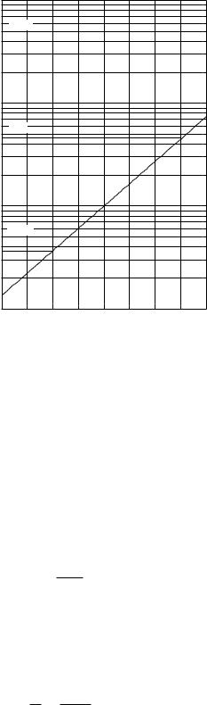
On semilog paper the vertical axis is marked in a logarithmic fashion. The graph can be plotted without having to calculate any logarithms. Figure 2.4 shows a plot of the exponential function of Fig. 2.2, for both positive and negative values of t. First, note how to read the vertical axis. A given distance along the axis always corresponds to the same multiplicative factor. Each cycle represents a factor of 10. To use the paper, it is necessary first to mark o the decades with the desired values. In Fig. 2.4 the decades have been marked 0.1, 1, 10, 100. The 6 that lies between 0.1 and 1 is 0.6; the 6 between 1 and 10 is 6.0; the 6 between 10 and 100 represents 60; and so forth. The paper can be imagined to go vertically forever in either direction; one never reaches zero. Figure 2.4 has two examples marked on it with dashed lines. The first shows that for t = −1.0, y = 0.36; the second shows that for t = +1.5, y = 4.5.

Semilog paper is most useful for plotting data that you suspect may have an exponential relationship. If the data plot as a straight line, your suspicions are confirmed.

	100
	7	←60
	6
	5
	4
	3
	2
	10
	7	←6
	6
	5
	4
y	3
	2
	1
	7	←0.6
	6
	5
	4
	3
	2
	0.1		-1.0	0.0	1.0	2.0
	-2.0
				t

FIGURE 2.4. A plot of the exponential function on semilog paper.

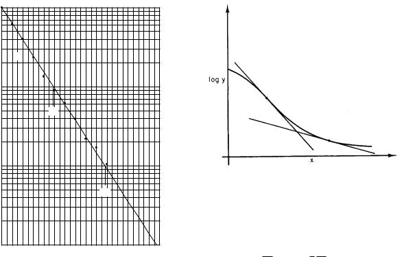
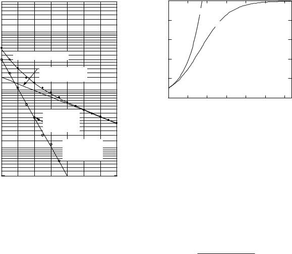
From the straight line, you can determine the value of b. Figure 2.5 is a plot of the intensity of light that passed through an absorber in a hypothetical example. The independent variable is absorber thickness x. The decay is exponential, except for the last few points, which may be high because of experimental error. (As the intensity of the light decreases, it becomes harder to measure accurately.) We wish to determine the decay constant in y = y0e−bx. One way to do it would be to note (dashed line A in Fig. 2.5) that the half-distance is 0.145 cm, so that, from Eq. 2.10,

b = 0.693 = 4.8 cm−1. 0.145

This technique can be inaccurate because it is di cult to read the graph accurately. It is more accurate to use a portion of the curve for which y changes by a factor of 10 or 100. The general relationship is y = y0ebx, where the value of b can be positive or negative. If two di erent values of x are selected, one can write

y2 = y0ebx2 = eb(x2−x1).

y1 y0ebx1

If y2/y1 = 10, then this equation has the form 10 = ebX10 where X10 = x2 − x1 when y2/y1 = 10. From a table of exponentials, bX10 = 2.303, so that

b =	2.303	.	(2.14)
	X10

	1
	7
	6
	5
	4
	3	A
	2
	0.1
Intensity	7
	6			B
	5
	4
	3
Relative
	2
	0.01
	7
	6
	5					C
	4
	3
	2
	0.001	0.2	0.4	0.6	0.8	1.0	1.2	1.4
	0.0

Thickness x, cm

FIGURE 2.5. A semilogarithmic plot of the intensity of light after it has passed through an absorber of thickness x.

The same procedure can be used to find b using a factor of 100 change in y:

b =	4.605	.	(2.15)
	X100
If the curve represents a	decaying		exponential, then

y2/y1 = 10 when x2 < x1, so that X10 = x2 − x1 is negative. Equation 2.14 then gives the negative value of b.

As an example, consider the exponential decay in Fig.

2.5. Using points B and C, we have x1 = 0.97, y1 = 10−2, x2 = 0.48, y2 = 10−1, X10 = 0.480 − 0.97 = −0.49. Therefore b = 2.303/(−0.49) = −4.7 cm−1, which is a more accurate determination than the one we made using the half-life.

2.4 Variable Rates

The equation dy/dx = by (or dy/dt = by) says that y grows or decays at a rate that is proportional to y. The constant b is the fractional rate of growth or decay. It is possible to define the fractional rate of growth or decay even if it is not constant but is a function of x:

b(x) =	1		dy	.	(2.16)
	y dx

Semilogarithmic graph paper can be used to analyze the curve even if b is not constant. Since d(ln y)/dy = 1/y,

2.4 Variable Rates

35

FIGURE 2.6. A semilogarithmic plot of y vs x when the decay rate is not constant. Each tangent line represents the instantaneous decay rate for that value of x.

the chain rule for evaluating derivatives gives

dxd (ln y) = y1 dxdy = b.

This means that b(x) is the slope of a plot of ln y vs. x. A semilogarithmic plot of y vs x is shown in Fig. 2.6. The straight line is tangent to the curve and decays with a constant rate equal to b(x) at the point of tangency. The value of b for the tangent line can be determined using the methods in the previous section. A second tangent line at a larger value of x in Fig. 2.6 has a smaller value of the decay rate.

If finite changes ∆x and ∆y have been measured, they may be used to estimate b(x) directly from Eq. 2.16. For example, suppose that y = 100, 000 people and that in ∆x = 1 year there is a change ∆y = −37. In this case ∆y is very small compared to y, so we can say that b = (1/y)(∆y/∆x) = −37 ×10−5. If the only cause of change in this population is deaths, the absolute value of b is called the death rate.

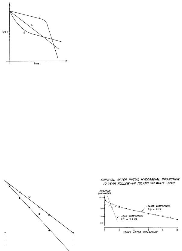
A plot of the number of people surviving in a population, all of whom have the same disease, can provide information about the prognosis for that disease. The death rate is equivalent to the decay constant. An example of such a plot is shown in Fig. 2.7. Curve A shows a disease for which the death rate is constant. Curve B shows a disease with an initially high death rate which decreases with time; if the patient survives the initial period, the prognosis is much better. Curve C shows a disease for which the death rate increases with time.

Surprisingly, there are a few diseases that have death rates independent of the duration of the disease (Zumo 1966). Any discussion of mortality should be made in terms of the surviving population, since any further deaths must come from that group. Nonetheless, one often finds results in the literature reported in terms of

36 2. Exponential Growth and Decay

FIGURE 2.7. Semilogarithmic plots of the fraction of a population surviving in three di erent diseases. The death rates (decay constants) depend on the duration of the disease.

the cumulative fraction of patients who have died. Figure 2.8 shows the survival of patients with congestive heart failure for a period of nine years. The data are taken from the Framingham study [McKee et al. (1971)]; the death rate is constant during this period. For a more detailed discussion of various possible survival distributions, see Clark (1975).

As long as b has a constant value, it makes no di erence what time is selected to be t = 0. To see this, suppose that the value of y decays exponentially with constant rate: y = y0e−bt. Consider two di erent time scales, shifted with respect to each other so that t = t0 + t. In terms of the shifted time t , the value of y is

y = y0e−bt = y0e−b(t −t0) = y0ebt0 e−bt .

1	9
	8
	7
													Females
	6
					Males
Surviving	5
	4
Fraction	3
	2
				Sex									b, yr-1										T1/2, yr
				Male							0.180											3.9
				Female							0.127											5.5
0.1
	0		2								4							6				8						10			12				14

T, years

FIGURE 2.8. Survival of patients with congestive heart failure. Data are from McKee et al. (1971).

This has the same form as the original expression for y(t). The value of y0 is y0ebt0 , which reflects the fact that t = 0 occurs at an earlier time than t = 0, so y0 > y0.

If the decay rate is not constant, then the origin of time becomes quite important. Usually there is something about the problem that allows t = 0 to be determined. Figure 2.9 shows survival after a heart attack (myocardial infarct). The time of the initial infarct defines t = 0; if the origin had been started two or three years after the infarct, the large initial death rate would not have been seen.

As long as the rate of increase can be written as a function of the independent variable, Eq. 2.16 can be rewritten as dy/y = b(x)dx. This can be integrated:

y2	dy			= x2 b(x) dx,
		y
					x1
y1
ln(y2/y1) =					x2
					b(x) dx,
					x1
		y2		= exp x2		b(x) dx .	(2.17)
		y1
					x1

If we can integrate the right-hand side analytically, numerically, or graphically, we can determine the ratio y2/y1.

2.5 Clearance

In some cases in physiology, the amount of a substance may decay exponentially because the rate of removal is proportional to the concentration of the substance (amount per unit volume) instead of to the total amount. For example, the rate at which the kidneys excrete a substance may be proportional to the concentration in the

FIGURE 2.9. The fraction of patients surviving after a myocardial infarction (heart attack) at t = 0. The curve labeled “Fast Component” plots 10 times the di erence between the survival curve and the extrapolated “Slow Component.” From B. Zumo , H. Hart, and L. Hellman (1966). Considerations of mortality in certain chronic diseases. Ann. Intern. Med. 64: 595–601. Reproduced by permission of Annals of Internal Medicine. Drawing courtesy of Prof. Zumo .

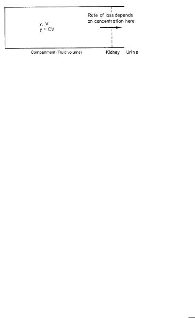
FIGURE 2.10. A case in which the rate of removal of a substance from the a fluid compartment depends on the concentration, not on the total amount of substance in the compartment. Increasing the compartment volume with the same concentration of the substance would not change the rate of removal.

blood that passes through the kidneys, while the total amount depends on the total fluid volume in which the substance is distributed. This is shown schematically in Fig. 2.10. The large box on the left represents the total fluid volume V . It contains a total amount of some substance, y. If the fluid is well mixed, the concentration is C = y/V . The removal process takes place only at the dashed line, at a rate proportional to C. The equation describing the change of y is

dy		y
	= −KC = −K			.	(2.18)
dt			V

The proportionality constant K is called the clearance. Its units are m3 s−1. The equation is the same as Eq. 2.6 if K/V is substituted for b. The solution is

y = y0e−(K/V )t.

(2.19)

The basic concept of clearance is best remembered in terms of Fig. 2.10. Other definitions are found in the literature. It sometimes takes considerable thought to show that the definitions are equivalent. A common definition in physiology books is “clearance is the volume of plasma from which y is completely removed per unit time.” To see that this definition is equivalent, imagine that y is removed from the body by removing a volume V of the plasma in which the concentration of y is C. The rate of loss of y is the concentration times the rate of volume removal:

dy		dV			C.	(2.20)
	=
			dt
dt		−

(dV /dt is negative for removal.) Comparison with Eq. 2.18 shows that |dV /dt| = K.

As long as the compartment containing the substance is well mixed, the concentration will decrease uniformly throughout the compartment as y is removed. The concentration also decreases exponentially:

C = C0e−(K/V )t.

(2.21)

An example may help to clarify the distinction between b and K. Suppose that the substance is distributed in

2.6 Multiple Decay Paths

37

a fluid volume V = 18 l. The substance has an initial concentration C0 = 3 mg l−1 and the clearance is K = 2 l h−1. The total amount is y0 = C0V = 3 × 18 = 54 mg. The fractional decay rate is b = K/V = 1/9 h−1. The equations for C and y are C = (3 mg l−1)e−t/9, y = (54 mg)e−t/9. At t = 0 the initial rate of removal is −dy/dt = 54/9 = 6 mg h−1.

Now double the fluid volume to V = 36 l without adding any more of the substance. The concentration falls to 1.5 mg l−1 although y0 is unchanged. The rate of removal is also cut in half, since it is proportional to K/V and the clearance is unchanged. The concentration and amount are now C = 1.5e−t/18, y = 54e−t/18. The initial rate of removal is dy/dt = 54/18 = 3 mg h−1. It is half as large as above, because C is now half as large.

If more of the substance were added along with the additional fluid, the initial concentration would be unchanged, but y0 would be doubled. The fractional decay rate would still be K/V = 1/18 h−1: C = 3.0e−t/18, y = 108e−t/18. The initial rate of disappearance would be dy/dt = 108/18 = 6 mg h−1. It is the same as in the first case, because the initial concentration is the same.

2.6 Multiple Decay Paths

It is possible to have several independent paths by which y can disappear. For example, there may be several competing ways by which a radioactive nucleus can decay; a radioactive isotope given to a patient may decay radioactively and be excreted biologically at the same time; a substance in the body can be excreted in the urine and metabolized by the liver; or patients may die of several di erent diseases.

In such situations the total decay rate b is the sum of the individual rates for each process, as long as the processes act independently and the rate of each is proportional to the present amount (or concentration) of y:

dy	= −b1y − b2y − b3y − · · ·	(2.22)
dt

= −(b1 + b2 + b3 + · · · )y = −by.

The equation for the disappearance of y is the same as before, with the total decay rate being the sum of the individual rates. The rate of disappearance of y by the ith process is not dy/dt but is −biy. Instead of decay rates, one can use half-lives. Since b = b1 + b2 + b3 + · · · , the total half-life T is given by

0.693

=

0.693

0.693

0.693

+

+

+ · · ·

T

T1

T2

T3

or

1

1

1

1

=

+

+

+ · · · .

(2.23)

T

T1

T2

T3

38 2. Exponential Growth and Decay

FIGURE 2.11. Sketch of the initial slope a and final value a/b of y when y(0) = 0.

2.7Decay Plus Input at a Constant Rate

Suppose that in addition to the removal of y from the system at a rate −by, y enters the system at a constant rate a, independent of y and t. The net rate of change of y is given by

dy	= a − by.	(2.24)
dt

It is often easier to write down a di erential equation describing a problem than it is to solve it. In this case the solution to the equation and the techniques for solving it are well known. However, a good deal can be learned about the solution by examining the equation itself. Suppose that y(0) = 0. Then the equation at t = 0 is dy/dt = a, and y initially grows at a constant rate a. As y builds up, the rate of growth decreases from this value because of the −by term. Finally, when a −by = 0, dy/dt is zero and y stops growing. This is enough information to make the sketch in Fig. 2.11.

The equation is solved in Appendix F. The solution is

y =	a	1 − e−bt .	(2.25)
	b

The derivative of y is dy/dt = ab (−1)(−b)e−bt = ae−bt. You can verify by substitution that Eq. 2.25 satisfies Eq. 2.24. The solution does have the properties sketched in Fig. 2.11, as you can see from Fig. 2.12. The initial value of dy/dt is a, and it decreases exponentially to zero. When t is large, the exponential term in y vanishes, leav-

ing y = a/b.

2.8Decay with Multiple Half-Lives and Fitting Exponentials

Sometimes y is a mixture of two or more quantities, each decaying at a constant rate. It might represent a mixture of radioactive isotopes, each decaying at its own rate. A biological example is the survival of patients after a myocardial infarct (Fig. 2.9). The death rate is not constant, and many models can be proposed to explain why. One possible model is that there are two distinct classes of

FIGURE 2.12. (a) Plot of y(t). (b) Plot of dy/dt.

patients immediately after the infarct. Each class has an associated death rate that is constant. After three years, virtually none of the subgroup with the higher death rate remains. Another model is that the death rate is higher right after the infarct for all patients. This higher death rate is due to causes associated with the myocardial injury: irritability of the muscle, arrhythmias in the heartbeat, the weakening of the heart wall at the site of the infarct, and so forth. After many months, the heart has healed, scar tissue has replaced the necrotic (dead) muscle, and deaths from these causes no longer occur.

Whatever the cause, it is sometimes useful to fit a set of experimental data with a sum of exponentials. It should be clear from the discussion of survival after myocardial infarction that simply fitting with an exponential or a sum of exponentials does not prove anything about the decay mechanism.

If y consists of two quantities, y1 and y2, each with its own decay rate, then

y = y1 + y2 = A1e−b1t + A2e−b2t.

(2.26)

Suppose that b1 > b2, so that y1 decays more rapidly than y2. After enough time has elapsed, y1 will be much less than y2, and its e ect on a semilog plot will be negligible. A typical plot of y is curve A in Fig. 2.13. Line B can then be drawn through the data and used to determine A2 and b2. This line is extrapolated back to earlier times, so that y2 can be subtracted from y to give an estimate for y1. For example, at point C (t = 4), y = 400, y2 = 300, and y1 = 100. At t = 0, y1 = 1500 − 500 = 1000. For times greater than 5 s, the curves for y and y2 are close together, and error in reading the graph produces considerable scatter in y1. When several values of y1 have

104
	7
	6
	5
	4
	3
	2
3		A: y = A		e-b1t + A e-b2t
			1		2
10
	7			B: Estimate that
	6			A2e-b2t = 500e-0.131t
	5
	4
y	3
	2
102				C: Typical
				subtraction
	7			of B from A:
				400-300 = 100
	6
	5
	4				D: Estimate that
	3				A1e	-b1t	=
	2				1000e-0.576t
101	0	2	4	6	8		10	12	14
					t

FIGURE 2.13. Fitting a curve with two exponentials.

been determined, line D is drawn, and parameters A1 and b1 are estimated.

This technique can be extended to several exponentials. However, it becomes increasingly di cult to extract meaningful parameters as more exponentials are used, because the estimated parameters for the short-lived terms are very sensitive to the initial guess for the parameters of the longest-lived term. For a discussion of this problem, see Riggs (1970), pp. 146–163.

2.9 The Logistic Equation

Exponential growth cannot go on forever. [This fact is often ignored by economists and politicians. Albert Bartlett has written extensively on this subject. You can find several references in The American Journal of Physics and The Physics Teacher. See the summary in Bartlett (2004).]

Sometimes a growing population will level o at some constant value. Other times the population will grow and then crash. One model that exhibits leveling o is the logistic model, described by the di erential equation

dy	= b0y	1 −	y	,	(2.27)
dt			y∞

where b0 and y∞ are constants. This equation has constant solutions y = 0 and y = y∞. If y y∞, then the

2.9 The Logistic Equation

39

1.0
	Exponential
0.8		Logistic
0.6
y
0.4
0.2
0.0	20	40	60	80	100	120
0
			t
FIGURE 2.14. Plot of the solution of the logistic equation
when y0 = 0.1, y∞ = 1.0, b0 = 0.0667. Exponential growth
with the same values of y0 and b0 is also shown.

equation is approximately dy/dt = b0y and y grows exponentially. As y becomes larger, the term in parentheses reduces the rate of increase of y, until y reaches the saturation value y∞. This might happen, for example, as the population begins to consume a significant fraction of the food supply, causing the birth rate to decrease or the mortality rate to increase.

If the initial value of y is y0, the solution of Eq. 2.27 is

y(t) =						1			(2.28)
		1	+		1		1	e−b0t
	y∞			y0		− y∞

= y0 y∞ . y0 + (y∞ − y0 )e−b0t

You can easily verify that y(0) = y0 and y(∞) = y∞. A plot of the solution is given in Fig. 2.14, along with exponential growth with the same value of b0.

Another way to think of Eq. 2.27 is that it has the form dy/dt = b(y)y, where b(y) = b0(1 − y/y∞) is now a function of the dependent variable y instead of the independent variable t. As y grows toward the asymptotic value, the growth rate b(y) decreases linearly to zero. The logistic model was an early and very important model for population growth. It provides good fits in a few cases, but there are now many more sophisticated models in population biology [Murray (2001)].

2.10Log–log Plots, Power Laws, and Scaling

2.10.1 Log-log Plots and Power Laws

This section considers the use of plots in which both scales are logarithmic: log–log plots. They are useful when x and y are related by the function

y = Bxn.

(2.29)

40 2. Exponential Growth and Decay

	10	y = x-1					y = x2			y = x
	7
	6
	5
	4									y = x1/2
	3
	2
y	1
	7
	6
	5
	4
	3
	2
	0.1	2	3	4	5	6 7	2	3	4	5	6 7
	0.1
							1				10
							x
FIGURE 2.15. Log-log plots of y = xn for di erent values of
n. When x = 1, y = 1 in every case.

Notice the di erence between this and the exponential function: here the independent variable x is raised to a constant power, while in the exponential case x (or t) is in the exponent. It also leads to a discussion of scaling, whereby simple physical arguments lead to important conclusions about the variations between species in size, shape, metabolic rate, and the like.

By taking logarithms of both sides of Eq. 2.29, we get

log y = log B + n log x.

(2.30)

This is a linear relationship between u = log y and v = log x:

u = const + nv.

(2.31)

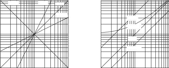
Therefore a plot of u vs v is a straight line with slope n. The slope can be positive or negative and need not be an integer. Figure 2.15 shows plots of y = x, y = x2, y = x1/2, and y = x−1. The slope can be determined from the graph by taking ∆u/∆v. The value of B is determined either by substituting particular values of y and x in Eq. 2.29 after n is known, or by determining the value of y when x = 1, in which case xn = 1 for any value of n, so n need not be known.

Figure 2.16 shows how the curves change when B is changed while n = 1. The curves are all parallel to one another. Multiplying by B is equivalent to adding a constant to log y.

If the expression is not of the form y = Bxn but has an added term, it will not plot as a straight line on log–log paper. Figure 2.16 also shows a plot of y = x + 1, which is not a straight line. (Of course, for very large values of x, log(x + 1) becomes nearly indistinguishable from log x, and the line appears straight.)

When the slope is constant, n can be determined from the slope ∆u/∆v measured with a ruler on the log–log

	10
	7
	6
	5
	4
	3					y = 4x
	2					y = x + 1
y	1
	7					y = x
	6
	5
	4					y = 0.5x
	3
	2
	0.1	2	3	4	5	6 7	2	3	4	5	6 7
	0.1
						1					10
						x

FIGURE 2.16. Log–log plots of y = Bx, showing how the curves shift on the paper as B changes. Since n = 1 for all the curves, they all have the same slope. There is also a plot of y = x + 1, to show that a polynomial does not plot as a straight line.

paper. When determining the slope in this way one must be sure that the length of a cycle is the same in each direction on the graph paper. To repeat the warning: it is easy to get a rough idea of the exponent from inspection of the slope of the log–log plot in Fig. 2.15 because on commercial log–log graph paper the distance spanned by a decade or cycle is the same on both axes. Some magazines routinely show log–log plots in which the distance spanned by a decade is not the same on both axes. Moreover, commercial graphing software does not impose this constraint on log–log plots, so it is becoming less and less likely that you can determine the exponent by glancing at the plot. Be careful!

When using a spreadsheet or other graphing software, it is often useful to make an extra column that contains the calculated variable ycalc = Axm with the values for A and m stored in two cells of the spreadsheet. If you plot this column as a line, and your real data as points without a line, then you can change the parameters while inspecting the graph to find the values that give the best fit.

An example of the use of a log–log plot is Poiseuille flow of fluid through a tube versus tube radius when the pressure gradient along the tube is constant (Problem 35). It was shown in Chapter 1 that an r4 dependence is expected.

2.10.2Food Consumption, Basal Metabolic Rate, and Scaling

Consider the relation of daily food consumption to body mass. This will introduce us to simple scaling arguments.

	104	Energy vs. Mass					Slope = 0.75
	7
	6	Height vs. Mass
(mm)	5						Slope = 0.62
	4
	3
or Height
	2
	103
(kcal/day)
	7
	6
	5						Slope = 0.33
	4
Energy
	3
	2
	102	2	3	4	5	6 7	2	3	4	5	6 7
	1
						10					100

Body Mass (kg)

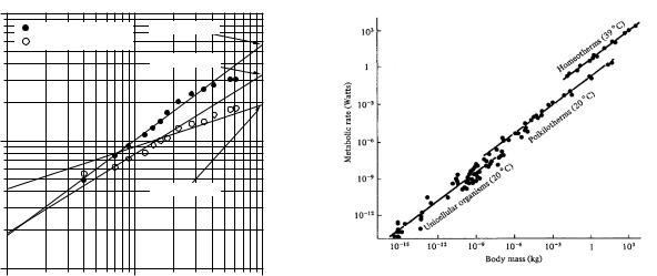
FIGURE 2.17. Plot of daily food requirement F and height H vs mass M for growing children. Data are from Kempe et al. (1970), p. 90.

As a first model, we might suppose that each kilogram of tissue has the same metabolic requirement, so that food consumption should be proportional to body mass. However, there is a problem with this argument. Most of the food that we consume is converted to heat. The various mechanisms to lose heat—radiation, convection and perspiration—are all roughly proportional to the surface area of the body rather than its mass. (This statement neglects the fact that considerable evaporation takes place through the lungs and that the body can control the rate of heat loss through sweating and shivering.) If all persons were the same shape, then the total surface area would be proportional to H2, where H is the height. The total volume and mass would be proportional to H3, so H would be proportional to M 1/3. Therefore the surface area would be proportional to (M 1/3)2 or M 2/3. (See Problem 40 for a discussion of other possible dependences of surface area on mass.) Figure 2.17 plots H and the total daily food requirement F vs body mass M for growing children [Kempe, Silver, and O’Brien (1970), p. 90].

Neither of the models proposed above fits the data very well. At early ages H is more nearly proportional to M 0.62 than to M 1/3. For older children, when the shape of the body has stopped changing, an M 0.33 dependence does fit better. This better fit occurs for masses greater than 23 kg, which correspond to ages over 6 years. The slope of the F (M ) curve is 0.75. This is less than the 1.0 of the model that food consumption is proportional to the mass and greater than the 0.67 of the model that food consumption is proportional to surface area.

This 3/4-power dependence is remarkable because it is seen across many species, from one-celled organisms to large mammals. It is called Kleiber’s law. Peters (1983) quotes work by Hemmingsen (1960) that shows the stan-

2.10 Log–log Plots, Power Laws, and Scaling

41

FIGURE 2.18. Plot of resting metabolic rate vs. body mass for many di erent organisms. Graph is from R. H. Peters (1983).

The Ecological Implications of Body Size. Cambridge, Cambridge University Press. Modified from A. M. Hemmingsen (1960). Energy metabolism as related to body size and respiratory surfaces, and its evolution. Reports of the Steno Memorial Hospital and Nordisk Insulin Laboratorium. 9 (Part II): 6–110. Used with permission.

dard metabolic rates for many species can be fitted by the following. The standard metabolic rate is in watts and mass in kilograms. (Standard means as close to resting or basal as possible.) For unicellular organisms at 20◦C,

Runicellular = 0.018M 0.751.

(2.32a)

The range of masses extended from 10−15 to 10−6 kg. For poikilotherms (organisms such as fish whose body temperature is the same as the surroundings) at 20 ◦C (masses from 10−8 to 102 kg),

Rpoikilotherm = 0.14M 0.751,

(2.32b)

and for homeotherms (animals that can maintain their body temperature independent of the surroundings) at 39◦C (masses from 10−2 to 103 kg),

Rhomeotherm = 4.1M 0.751.

(2.32c)

Peters’s graph is shown in Fig. 2.18.

The 3/4-power dependence has been widely accepted; however, some recent analyses of the data, such as White and Seymour (2003), support a 2/3 power dependence. Even more recent studies a rm a 3/4 power [Savage et al. (2004)].

A number of models have been proposed to explain a 3/4-power dependence [McMahon (1973); Peters (1983); West et al. (1999); Banavar et al. (1999)]. West et al. argue that the 3/4-power dependence is universal: they derive it from a model that supplies nutrients through a branching network that reaches all parts of the organism, minimizes the energy required for distribution,

42 2. Exponential Growth and Decay

and ends in capillaries (or terminal xylem in plants) that are all the same size. Whether it is universal is still debated [Kozlowski and Konarzewski (2004)]. West and Brown (2004) review quarter-power scaling in a variety of circumstances.

We will discuss temperature dependence in Chapter 3.

Symbols Used in Chapter 2

Symbol	Use	Units	First
			used on
			page
a	Rate of input of a	s−1	38
	substance
b, b0	Rate of growth or decay	s−1,h−1	31
c1, c2	Constants		34
f	Fraction		33
m, n	Exponent in power law		39
	relationship
t	Time	s	32
u	Logarithm of dependent		34
	variable
v	Logarithm of independent		40
	variable
x	General independent		33
	variable
y	General dependent		32
	variable
y	Amount of substance in	kg, mg	37
	plasma
x0,y0	Initial value of x or y		32
y∞	Saturation value of y		39
A	Constant		38
B	Constant		39
C	Concentration	kg m−3, etc.	37
F	Food requirement	kcal day−1	41
H	Body height	m	41
K	Clearance	m3 s−1	37
M	Body mass	kg	41
N	Number of compoundings		32
	per year
R	Standard metabolic rate	W	41
T1/2	Half-life	s, etc.	34
T2	Doubling time	s	34
V	Volume	m3	37
X10	Change in x for a		34
	factor-of-10 change in y
X100	Change in x for a		35
	factor-of-100 change in y

Problems

Section 2.1

Problem 1 Suppose that you are 20 years old and have an annual income of $20,000. You plan to work for 40 years. If inflation takes place at a rate of 3% per year, what income would you need at age 60 to have the same

buying power you have now? Ignore taxes. Make the calculation assuming that (a) inflation is 3% and occurs once a year and (b) inflation is continuous but at a 3% annual rate.

Problem 2 The number e is defined by limn→∞(1 + 1/n)n.

(a)Calculate values of (1+1/n)n for n = 1, 2, 4, 8, and

16.

(b)Use the binomial formula (1 + a)n = 1 + na +

n(n−1) 2			n(n−1)(n−2)			3		x
		a +			a		+ · · · to obtain a series for e		=
2!			3!n
limn→∞(1 + x/n)				. [See also Appendix D, Eq. D.3.]

Problem 3 A child with acute lymphocytic leukemia (ALL) has approximately 1012 leukemic cells when the disease is clinically apparent.

(a)If a cell is about 8 µm in diameter, estimate the total mass of leukemic cells.

(b)Curing the disease requires killing every single cell. The doubling time for the cells is about 5 days. If all cells were killed except for one, how long would it take for the disease to become apparent again?

(c)Suppose that chemotherapy reduces the number of cells to 109 and there are no changes of ALL cell properties (no mutations). How long a remission would you expect? What if the number were reduced to 106?

Problem 4 Suppose that tumor cells within the body reproduce at rate r, so that the number is given by y = y0ert. Each time a chemotherapeutic agent is given it destroys a fraction f of the cells then existing. Make a semilog plot showing y as a function of time for several administrations of the drug, separated by time T . What di erent cases must you consider for the relation among f , T , and r?

Problem 5 An exponentially growing culture of bacteria increases from 106 to 5 × 108 cells in 6 h. What is the time between successive cell divisions if there is no cell mortality?

Problem 6 The following data on railroad tracks were obtained from R. H. Romer [(1991). The mathematics of exponential growth—keep it simple, Phys. Teach. 9: 344–

345]:
Year	Miles of track
1860	30, 626
1870	52, 922
1880	93, 262
1890	166, 703

(a)What is the doubling time?

(b)Estimate the surface area of the contiguous United States. Assume that a railroad roadbed is 7 m wide. In what year would an extrapolation predict that the surface of the United States would be completely covered with railroad track?