

Brereton Chemometrics
.pdfEXPERIMENTAL DESIGN |
99 |
|||
|
|
|
|
|
|
|
|
|
|
|
|
|
|
|
Factor2 |
Factor 1
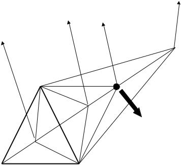
Figure 2.38
Progress of a fixed sized simplex
In the case illustrated in Figure 2.37, this would simply involve reflecting point 2 in the centroid of points 1 and 3. Keep these new conditions together with the worst and the k − 1 best responses from the previous simplex. The second worst response from the previous simplex is rejected, so in the case of three factors, we keep old responses 1, 3 and the new one, rather than old responses 2, 3 and the new one.
6.Check for convergence. When the simplex is at an optimum it normally oscillates around in a triangle or hexagon. If the same conditions reappear, stop. There are a variety of stopping rules, but it should generally be obvious when optimisation has been achieved. If you are writing a robust package you will be need to take a lot of rules into consideration, but if you are doing the experiments manually it is normal simply to check what is happening.
The progress of a fixed sized simplex is illustrated in Figure 2.38.
2.6.2 Elaborations
There are many elaborations that have been developed over the years. One of the most important is the k + 1 rule. If a vertex has remained part of the simplex for k + 1 steps, perform the experiment again. The reason for this is that response surfaces may be noisy, so an unduly optimistic response could have been obtained because of experimental error. This is especially important when the response surface is flat near the optimum. Another important issue relates to boundary conditions. Sometimes there are physical reasons why a condition cannot cross a boundary, an obvious case being a negative concentration. It is not always easy to deal with such situations, but it is possible to use step 5 rather than step 4 above under such circumstances. If the simplex constantly tries to cross a boundary either the constraints are slightly unrealistic and so should be changed, or the behaviour near the boundary needs further investigation. Starting a new simplex near the boundary with a small step size may solve the problem.
100 |
CHEMOMETRICS |
|
|
2.6.3 Modified Simplex
A weakness with the standard method for simplex optimisation is a dependence on the initial step size, which is defined by the initial conditions. For example, in Figure 2.37 we set a very small step size for both variables; this may be fine if we are sure we are near the optimum, but otherwise a bigger triangle would reach the optimum quicker, the problem being that the bigger step size may miss the optimum altogether. Another method is called the modified simplex algorithm and allows the step size to be altered, reduced as the optimum is reached, or increased when far from the optimum.
For the modified simplex, step 4 of the fixed sized simplex (Section 2.6.1) is changed as follows. A new response at point xtest is determined, where the conditions are obtained as for fixed sized simplex. The four cases below are illustrated in Figure 2.39.
(a)If the response is better than all the other responses in the previous simplex, i.e. ytest > yk+1 then expand the simplex, so that
xnew = c + α(c − x1)
where α is a number greater than 1, typically equal to 2.
(b)If the response is better than the worst of the other responses in the previous simplex, but worst than the second worst, i.e. y1 < ytest < y2, then contract the
Case a
Case b
Case d
Case c
3
Test conditions
1 |
2 |
Figure 2.39
Modified simplex. The original simplex is indicated in bold, with the responses ordered from 1 (worst) to 3 (best). The test conditions are indicated
EXPERIMENTAL DESIGN |
101 |
|
|
simplex but in the direction of this new response:
xnew = c + β(c − x1)
where β is a number less than 1, typically equal to 0.5.
(c)If the response is worse than the other responses, i.e. ytest < y1, then contract the simplex but in the opposite direction of this new response:
xnew = c − β(c − x1)
where β is a number less than 1, typically equal to 0.5.
(d) In all other cases simply calculate
xnew = xtest = c + c − x1
as in the normal (fixed-sized) simplex.
Then perform another experiment at xnew and keep this new experiment plus the k(=2) best experiments from the previous simplex to give a new simplex.
Step 5 still applies: if the value of the response at the new vertex is less than that of the remaining k responses, return to the original simplex and reject the second best response, repeating the calculation as above.
There are yet further sophistications such as the supermodified simplex, which allows mathematical modelling of the shape of the response surface to provide guidelines as to the choice of the next simplex. Simplex optimisation is only one of several computational approaches to optimisation, including evolutionary optimisation and steepest ascent methods. However, it has been much used in chemistry, largely owing to the work of Deming and colleagues, being one of the first systematic approaches applied to the optimisation of real chemical data.
2.6.4 Limitations
In many well behaved cases, simplex performs well and is an efficient approach for optimisation. There are, however, a number of limitations.
•If there is a large amount of experimental error, then the response is not very reproducible. This can cause problems, for example, when searching a fairly flat response surface.
•Sensible initial conditions and scaling (coding) of the factors are essential. This can only come form empirical chemical knowledge.
•If there are serious discontinuities in the response surface, this cannot always be taken into account.
•There is no modelling information. Simplex does not aim to predict an unknown response, produce a mathematical model or test the significance of the model using ANOVA. There is no indication of the size of interactions or related effects.
There is some controversy as to whether simplex methods should genuinely be considered as experimental designs, rather than algorithms for optimisation. Some statisticians often totally ignore this approach and, indeed, many books and courses of

102 |
CHEMOMETRICS |
|
|
experimental design in chemistry will omit simplex methods altogether, concentrating exclusively on approaches for mathematical modelling of the response surface. However, engineers and programmers have employed simplex and related approaches for optimisation for many years, and these methods have been much used, for example, in spectroscopy and chromatography, and so should be considered by the chemist. As a practical tool where the detailed mathematical relationship between response and underlying variables is not of primary concern, the methods described above are very valuable. They are also easy to implement computationally and to automate and simple to understand.
Problems
Problem 2.1 A Two Factor, Two Level Design
Section 2.2.3 Section 2.3.1
The following represents the yield of a reaction recorded at two catalyst concentrations and two reaction times:
Concentration (mM) |
Time (h) |
Yield (%) |
|
|
|
0.1 |
2 |
29.8 |
0.1 |
4 |
22.6 |
0.2 |
2 |
32.6 |
0.2 |
4 |
26.2 |
|
|
|
1.Obtain the design matrix from the raw data, D, containing four coefficients of the form
y= b0 + b1x1 + b2x2 + b12x1x2
2.By using this design matrix, calculate the relationship between the yield (y) and the two factors from the relationship
b = D−1.y
3.Repeat the calculations in question 2 above, but using the coded values of the design matrix.
Problem 2.2 Use of a Fractional Factorial Design to Study Factors That Influence NO Emissions in a Combustor
Section 2.2.3 Section 2.3.2
It is desired to reduce the level of NO in combustion processes for environmental reasons. Five possible factors are to be studied. The amount of NO is measured as mg MJ−1 fuel. A fractional factorial design was performed. The following data were obtained, using coded values for each factor:

EXPERIMENTAL DESIGN |
|
|
|
|
103 |
||
|
|
|
|
|
|
|
|
|
|
|
|
|
|
|
|
|
Load |
Air: fuel |
Primary |
NH3 |
Lower |
NO |
|
|
|
ratio |
air (%) |
(dm3 h−1) |
secondary air (%) |
(mg MJ−1) |
|
|
−1 |
−1 |
−1 |
−1 |
1 |
109 |
|
1 |
−1 |
−1 |
1 |
−1 |
26 |
|
|
|
−1 |
1 |
−1 |
1 |
−1 |
31 |
|
1 |
1 |
−1 |
−1 |
1 |
176 |
|
|
|
−1 |
−1 |
1 |
1 |
1 |
41 |
|
1 |
−1 |
1 |
−1 |
−1 |
75 |
|
|
|
−1 |
1 |
1 |
−1 |
−1 |
106 |
|
|
1 |
1 |
1 |
1 |
1 |
160 |
|
1.Calculate the coded values for the intercept, the linear and all two factor interaction terms. You should obtain a matrix of 16 terms.
2.Demonstrate that there are only eight unique possible combinations in the 16 columns and indicate which terms are confounded.
3.Set up the design matrix inclusive of the intercept and five linear terms.
4.Determine the six terms arising from question 3 using the pseudo-inverse. Interpret the magnitude of the terms and comment on their significance.
5.Predict the eight responses using yˆ = D.b and calculate the percentage root mean square error, adjusted for degrees of freedom, relative to the average response.
Problem 2.3 Equivalence of Mixture Models
Section 2.5.2.2
The following data are obtained for a simple mixture design:
Factor 1 |
Factor 2 |
Factor 3 |
Response |
|
|
|
|
1 |
0 |
0 |
41 |
0 |
1 |
0 |
12 |
0 |
0 |
1 |
18 |
0.5 |
0.5 |
0 |
29 |
0.5 |
0 |
0.5 |
24 |
0 |
0.5 |
0.5 |
17 |
|
|
|
|
1. The data are to be fitted to a model of the form
y = b1x1 + b2x2 + b3x3 + b12x1x2 + b13x1x3 + b23x2x3
Set up the design matrix, and by calculating D−1.y determine the six coefficients. 2. An alternative model is of the form
y = a0 + a1x1 + a2x2 + a11x12 + a22x22 + a12x1x2
Calculate the coefficients for this model.
3.Show, algebraically, the relationship between the two sets of coefficients, by substituting
x3 = 1 − x1 − x2

104 |
CHEMOMETRICS |
|
|
into the equation for the model 1 above. Verify that the numerical terms do indeed obey this relationship and comment.
Problem 2.4 Construction of Mixture Designs
Section 2.5.3 Section 2.5.4
1.How many experiments are required for {5, 1}, {5, 2} and {5, 3} simplex lattice designs?
2.Construct a {5, 3} simplex lattice design.
3.How many combinations are required in a full five factor simplex centroid design? Construct this design.
4.Construct a {3, 3} simplex lattice design.
5.Repeat the above design using the following lower bound constraints:
x1 ≥ 0.0 x2 ≥ 0.3 x3 ≥ 0.4
Problem 2.5 Normal Probability Plots
Section 2.2.4.5
The following is a table of responses of eight experiments at coded levels of three variables, A, B and C:
A |
B |
C |
response |
|
|
|
|
−1 |
−1 |
−1 |
10 |
1 |
−1 |
−1 |
9.5 |
−1 |
1 |
−1 |
11 |
1 |
1 |
−1 |
10.7 |
−1 |
−1 |
1 |
9.3 |
1 |
−1 |
1 |
8.8 |
−1 |
1 |
1 |
11.9 |
1 |
1 |
1 |
11.7 |
1.It is desired to model the intercept and all single, two and three factor coefficients. Show that there are only eight coefficients and explain why squared terms cannot be taken into account.
2.Set up the design matrix and calculate the coefficients. Do this without using the pseudo-inverse.
3.Excluding the intercept term, there are seven coefficients. A normal probability
plot can be obtained as follows. First, rank the seven coefficients in order. Then, for each coefficient of rank p calculate a probability (p − 0.5)/7. Convert these probabilities into expected proportions of the normal distribution for a reading of appropriate rank using an appropriate function in Excel. Plot the values of each of the seven effects (horizontal axis) against the expected proportion of normal distribution for a reading of given rank.

EXPERIMENTAL DESIGN |
105 |
|
|
4.From the normal probability plot, several terms are significant. Which are they?
5.Explain why normal probability plots work.
Problem 2.6 Use of a Saturated Factorial Design to Study Factors in the Stability of a Drug
Section 2.3.1 Section 2.2.3
The aim of the study is to determine factors that influence the stability of a drug, diethylpropion, as measured by HPLC after 24 h. The higher the percentage, the better is the stability. Three factors are considered:
Factor |
Level (−) |
Level (+) |
Moisture (%) |
57 |
75 |
Dosage form |
Powder |
Capsule |
Clorazepate (%) |
0 |
0.7 |
|
|
|
A full factorial design is performed, with the following results, using coded values for each factor:
Factor 1 |
Factor 2 |
Factor 3 |
Response |
|
|
|
|
−1 |
−1 |
−1 |
90.8 |
1 |
−1 |
−1 |
88.9 |
−1 |
1 |
−1 |
87.5 |
1 |
1 |
−1 |
83.5 |
−1 |
−1 |
1 |
91.0 |
1 |
−1 |
1 |
74.5 |
−1 |
1 |
1 |
91.4 |
1 |
1 |
1 |
67.9 |
1.Determine the design matrix corresponding to the model below, using coded values throughout:
y= b0 + b1x1 + b2x2 + b3x3 + b12x1x2 + b13x1x3 + b23x2x3 + b123x1x2x3
2.Using the inverse of the design matrix, determine the coefficients b = D−1.y.
3.Which of the coefficients do you feel are significant? Is there any specific interaction term that is significant?
4.The three main factors are all negative, which, without considering the interaction terms, would suggest that the best response is when all factors are at their lowest level. However, the response for the first experiment is not the highest, and this suggests that for best performance at least one factor must be at a high level. Interpret this in the light of the coefficients.
5.A fractional factorial design could have been performed using four experiments. Explain why, in this case, such a design would have missed key information.
6.Explain why the inverse of the design matrix can be used to calculate the terms in the model, rather than using the pseudo-inverse b = (D .D)−1.D .y. What changes in the design or model would require using the pseudo-inverse in the calculations?

106 |
CHEMOMETRICS |
|
|
7.Show that the coefficients in question 2 could have been calculated by multiplying the responses by the coded value of each term, summing all eight values, and dividing by eight. Demonstrate that the same answer is obtained for b1 using both methods of calculation, and explain why.
8.From this exploratory design it appears that two major factors and their interaction are most significant. Propose a two factor central composite design that could be used to obtain more detailed information. How would you deal with the third original factor?
Problem 2.7 Optimisation of Assay Conditions for tRNAs Using a Central Composite Design
Section 2.4 Section 2.2.3 Section 2.2.2 Section 2.2.4.4 Section 2.2.4.3
The influence of three factors, namely pH, enzyme concentration and amino acid concentration, on the esterification of tRNA arginyl-tRNA synthetase is to be studied by counting the radioactivity of the final product, using 14C-labelled arginine. The higher is the count, the better are the conditions.
The factors are coded at five levels as follows:
|
|
|
|
Level |
|
|
|
|
|
|
|
|
|
|
|
−1.7 |
−1 |
0 |
1 |
1.7 |
Factor 1: enzyme (µg protein) |
3.2 |
6.0 |
10.0 |
14.0 |
16.8 |
|
Factor 2: arginine (pmol) |
860 |
1000 |
1200 |
1400 |
1540 |
|
Factor 3: pH |
6.6 |
7.0 |
7.5 |
8.0 |
8.4 |
|
|
|
|
|
|
|
|
The results of the experiments are as follows:
Factor 1 |
Factor 2 |
Factor 3 |
Counts |
|
|
|
|
1 |
1 |
1 |
4930 |
1 |
1 |
−1 |
4810 |
1 |
−1 |
1 |
5128 |
1 |
−1 |
−1 |
4983 |
−1 |
1 |
1 |
4599 |
−1 |
1 |
−1 |
4599 |
−1 |
−1 |
1 |
4573 |
−1 |
−1 |
−1 |
4422 |
1.7 |
0 |
0 |
4891 |
−1.7 |
0 |
0 |
4704 |
0 |
1.7 |
0 |
4566 |
0 |
−1.7 |
0 |
4695 |
0 |
0 |
1.7 |
4872 |
0 |
0 |
−1.7 |
4773 |
0 |
0 |
0 |
5063 |
0 |
0 |
0 |
4968 |
0 |
0 |
0 |
5035 |
|
|
|
|

EXPERIMENTAL DESIGN |
107 |
|
|
Factor 1 |
Factor 2 |
Factor 3 |
Counts |
|
|
|
|
0 |
0 |
0 |
5122 |
0 |
0 |
0 |
4970 |
0 |
0 |
0 |
4925 |
|
|
|
|
1. Using a model of the form
yˆ = b0 + b1x1 + b2x2 + b3x3 + b11x12 + b22x22 + b33x32
+ b12x1x2 + b13x1x3 + b23x2x3
set up the design matrix D.
2.How many degrees-of-freedom are required for the model? How many are available for replication and so how many left to determine the significance of the lack-of-fit?
3.Determine the coefficients of the model using the pseudo-inverse b = (D .D)−1.D .y where y is the vector of responses.
4.Determine the 20 predicted responses by yˆ = D.b, and so the overall sum of square residual error, and the root mean square residual error (divide by the residual degrees of freedom). Express the latter error as a percentage of the standard deviation of the measurements. Why is it more appropriate to use a standard deviation rather than a mean in this case?
5.Determine the sum of square replicate error, and so, from question 4, the sum of square lack-of-fit error. Divide the sum of square residual, lack-of-fit and replicate errors by their appropriate degrees of freedom and so construct a simple ANOVA table with these three errors, and compute the F -ratio.
6.Determine the variance of each of the 10 parameters in the model as follows. Compute the matrix (D .D)−1 and take the diagonal elements for each parameter. Multiply these by the mean square residual error obtained in question 5.
7.Calculate the t-statistic for each of the 10 parameters in the model, and so determine which are most significant.
8.Select the intercept and five other most significant coefficients and determine a new model. Calculate the new sum of squares residual error, and comment.
9.Using partial derivatives, determine the optimum conditions for the enzyme assay using coded values of the three factors. Convert these to the raw experimental conditions.
Problem 2.8 Simplex Optimisation
Section 2.6
Two variables, a and b, influence a response y. These variables may, for example, correspond to pH and temperature, influencing level of impurity. It is the aim of optimisation to find the values of a and b that give the minimum value of y.
The theoretical dependence of the response on the variables is
y = 2 + a2 − 2a + 2b2 − 3b + (a − 2)(b − 3)

108 CHEMOMETRICS
Assume that this dependence is unknown in advance, but use it to generate the response for any value of the variables. Assume there is no noise in the system.
1. |
Using partial derivatives show that the |
minimum value of y is obtained when |
||
|
a = 15/7 and compute the value of b and y at this minimum. |
|||
2. |
Perform simplex optimisation using as a starting point |
|||
|
|
|
|
|
|
|
a |
b |
|
|
|
|
|
|
|
0 |
0 |
|
|
|
1 |
0 |
|
|
|
0.5 |
0.866 |
|
|
|
|
|
|
|
This is done by generating the equation for y and watching how y changes with each new set of conditions a and b. You should reach a point where the response oscillates; although the oscillation is not close to the minimum, the values of a and b giving the best overall response should be reasonable. Record each move of the simplex and the response obtained.
3.What are the estimated values of a, b and y at the minimum and why do they differ from those in question 1?
4.Perform a simplex using a smaller step-size, namely starting at
a |
b |
|
|
0 |
0 |
0.5 |
0 |
0.25 |
0.433 |
|
|
What are the values of a, b and y and why are they much closer to the true minimum?
Problem 2.9 Error Analysis for Simple Response Modelling
Section 2.2.2 Section 2.2.3
The follow represents 12 experiments involving two factors x1 and x2, together with the response y:
x1 |
x2 |
y |
0 |
0 |
5.4384 |
0 |
0 |
4.9845 |
0 |
0 |
4.3228 |
0 |
0 |
5.2538 |
−1 |
−1 |
8.7288 |
−1 |
1 |
0.7971 |
1 |
−1 |
10.8833 |