Brereton Chemometrics

PATTERN RECOGNITION	211

Table 4.10 Raw data for Section 4.3.6.

	A	B	C	D	E	F	G	H
1	0.318	0.413	0.335	0.196	0.161	0.237	0.290	0.226
2	0.527	0.689	0.569	0.346	0.283	0.400	0.485	0.379
3	0.718	0.951	0.811	0.521	0.426	0.566	0.671	0.526
4	0.805	1.091	0.982	0.687	0.559	0.676	0.775	0.611
5	0.747	1.054	1.030	0.804	0.652	0.695	0.756	0.601
6	0.579	0.871	0.954	0.841	0.680	0.627	0.633	0.511
7	0.380	0.628	0.789	0.782	0.631	0.505	0.465	0.383
8	0.214	0.402	0.583	0.635	0.510	0.363	0.305	0.256
9	0.106	0.230	0.378	0.440	0.354	0.231	0.178	0.153
10	0.047	0.117	0.212	0.257	0.206	0.128	0.092	0.080

1

2

3

4

5

6

7

8

9

10

Datapoint

Figure 4.15

Profile for data in Table 4.10

data packages that have been designed primarily by statisticians. What is mainly interesting in traditional studies is the deviation around a mean, for example, how do the mean characteristics of a forged banknote vary? What is an ‘average’ banknote? In chemistry, however, we are often (but by no means exclusively) interested in the deviation above a baseline, such as in spectroscopy. It is also crucial to recognise that some of the traditional properties of principal components, such as the correlation coefficient between two score vectors being equal to zero, are no longer valid for raw data. Despite this, there is often good chemical reason for using applying PCA to the raw data.

	212										CHEMOMETRICS
		0.4
							8
		0.3			9				7
		0.2		10
											6
		0.1
	PC2	0
		0		0.5		1		1.5		2		2.5
											5
		−0.1
						1
		−0.2						2			4
		−0.3								3
		−0.4
							PC1
		0.8
		0.6								D
		0.4						E
		0.2
											C
	PC2	0							F			.
		0	0.05	0.1	0.15	0.2	0.25	0.3	0.35	0.4	0.45
												0.5
		−0.2						H
									G
		−0.4									B
									A
		−0.6
							PC1

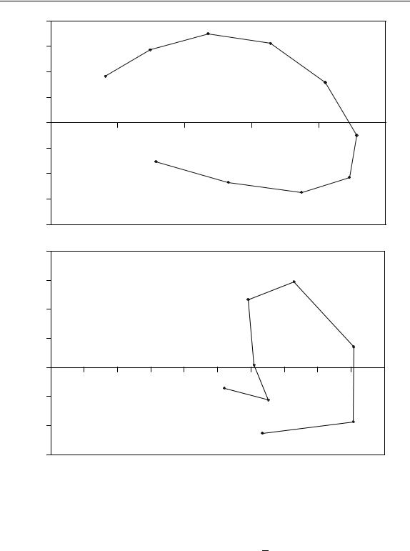
Figure 4.16

Scores and loadings plots of first two PCs of data in Table 4.10

4.3.6.3 Mean Centring

It is, however, possible to mean centre the columns by subtracting the mean of each column (or variable) so that

cen xij = xij − xj

PATTERN RECOGNITION	213

Table 4.11 Mean-centred data corresponding to Table 4.10.

	A	B	C	D	E	F	G	H
1	−0.126	−0.231	−0.330	−0.355	−0.285	−0.206	−0.175	−0.146
2	0.083	0.045	−0.095	−0.205	−0.163	−0.042	0.020	0.006
3	0.273	0.306	0.146	−0.030	−0.020	0.123	0.206	0.153
4	0.360	0.446	0.318	0.136	0.113	0.233	0.310	0.238
5	0.303	0.409	0.366	0.253	0.206	0.252	0.291	0.229
6	0.135	0.226	0.290	0.291	0.234	0.185	0.168	0.139
7	−0.064	−0.017	0.125	0.231	0.184	0.062	0.000	0.010
8	−0.230	−0.243	−0.081	0.084	0.064	−0.079	−0.161	−0.117
9	−0.338	−0.414	−0.286	−0.111	−0.093	−0.212	−0.287	−0.220
10	−0.397	−0.528	−0.452	−0.294	−0.240	−0.315	−0.373	−0.292

The result is presented in Table 4.11. Note that the sum of each column is now zero. Almost all traditional statistical packages perform this operation prior to PCA, whether desired or not. The PC plots are presented in Figure 4.17.

The most obvious difference is that the scores plot is now centred around the origin. However, the relative positions of the points in both graphs change slightly, the largest effect being on the loadings in this case. In practice, mean centring can have a large influence, for example if there are baseline problems or only a small region of the data is recorded. The reasons why the distortion is not dramatic in this case is that the averages of the eight variables are comparable in size, varying from 0.38 to 0.64. If there is a much wider variation this can change the patterns of both scores and loadings plots significantly, so the scores of the mean-centred data are not necessarily the ‘shifted’ scores of the original dataset.

Mean centring often has a significant influence on the relative size of the first eigenvalue, which is reduced dramatically in size, and can influence the apparent number of significant components in a dataset. However, it is important to recognise that in signal analysis the main feature of interest is variation above a baseline, so mean centring is not always appropriate in a physical sense in certain areas of chemistry.

4.3.6.4 Standardisation

Standardisation is another common method for data scaling and occurs after mean centring; each variable is also divided by its standard deviation:

stn x				xij −				j
						x
ij =
		I		(xij					j )2	/I
			1		−		x
	i
		=

see Table 4.12 for our example. Note an interesting feature that the sum of squares of each column equals 10 (which is the number of objects in the dataset), and note also that the ‘population’ rather than ‘sample’ standard deviation (see Appendix A.3.1.2) is employed. Figure 4.18 represents the new graphs. Whereas the scores plot hardly changes in appearance, there is a dramatic difference in the appearance of the loadings. The reason is that standardisation puts all the variables on approximately the same scale. Hence variables (such as wavelengths) of low intensity assume equal significance

214							CHEMOMETRICS
				0.4
				0.3	7
				8
				0.2		6
			9
				0.1
PC2							5
		10 −1		0
	−1.5			−0.5	0	0.5	1
				−0.1			4
				−0.2
					2	3
			1	−0.3
				−0.4
				PC1
	0.8
	0.6			D
				E
	0.4
	0.2					C
PC2				F
	0
	0	0.1	0.2	0.3	0.4	0.5	0.6
−0.2				H	G
							B
−0.4					A
−0.6
				PC1

Figure 4.17

Scores and loadings plots of first two PCs of data in Table 4.11

to those of high intensity. Note that now the variables are roughly the same distance away from the origin, on an approximate circle (this looks distorted simply because the horizontal axis is longer than the vertical axis), because there are only two significant components. If there were three significant components, the loadings would fall roughly on a sphere, and so on as the number of components is increased. This simple

PATTERN RECOGNITION	215

Table 4.12 Standardised data corresponding to Table 4.10.

	A	B	C	D	E	F	G	H
1	−0.487	−0.705	−1.191	−1.595	−1.589	−1.078	−0.760	−0.818
2	0.322	0.136	−0.344	−0.923	−0.909	−0.222	0.087	0.035
3	1.059	0.933	0.529	−0.133	−0.113	0.642	0.896	0.856
4	1.396	1.361	1.147	0.611	0.629	1.218	1.347	1.330
5	1.174	1.248	1.321	1.136	1.146	1.318	1.263	1.277
6	0.524	0.690	1.046	1.306	1.303	0.966	0.731	0.774
7	−0.249	−0.051	0.452	1.040	1.026	0.326	0.001	0.057
8	−0.890	−0.740	−0.294	0.376	0.357	−0.415	−0.698	−0.652
9	−1.309	−1.263	−1.033	−0.497	−0.516	−1.107	−1.247	−1.228
10	−1.539	−1.608	−1.635	−1.321	−1.335	−1.649	−1.620	−1.631

visual technique is also a good method for confirming that there are two significant components in a dataset.

Standardisation can be important in real situations. Consider, for example, a case where the concentrations of 30 metabolites are monitored in a series of organisms. Some metabolites might be abundant in all samples, but their variation is not very significant. The change in concentration of the minor compounds might have a significant relationship to the underlying biology. If standardisation is not performed, PCA will be dominated by the most intense compounds.

In some cases standardisation (or closely related scaling) is an essential first step in data analysis. In case study 2, each type of chromatographic measurement is on a different scale. For example, the N values may exceed 10 000, whereas k’ rarely exceeds 2. If these two types of information were not standardised, PCA will be dominated primarily by changes in N, hence all analysis of case study 2 in this chapter involves preprocessing via standardisation. Standardisation is also useful in areas such as quantitative structure–property relationships, where many different pieces of information are measured on very different scales, such as bond lengths and dipoles.

	4.3.6.5 Row Scaling
	Scaling the rows to a constant total,	usually 1 or 100, is a common procedure,
	for example		xij
	cs xij	=
			J

xij

j =1

Note that some people use term ‘normalisation’ in the chemometrics literature to define this operation, but others define normalised vectors (see Section 4.3.2 and Chapter 6, Section 6.2.2) as those whose sum of squares rather than sum of elements equals one. In order to reduce confusion, in this book we will restrict the term normalisation to the transformation that sets the sum of squares to one.

Scaling the rows to a constant total is useful if the absolute concentrations of samples cannot easily be controlled. An example might be biological extracts: the precise amount of material might vary unpredictably, but the relative proportions of each chemical can be measured. This method of scaling introduces a constraint which is often called closure. The numbers in the multivariate data matrix are proportions and

216									CHEMOMETRICS
						1.5
					8		7
						1			6
			9
						0.5
PC2		10				0					5
	−5	−4	−3	−2	−1	0	1	2	3		4
						−0.5
										4
						−1
			1					3
						2
						−1.5
						PC1
0.8
0.6								D	E
0.4
0.2
PC2										C
	0
	0	0.05	0.1		0.15	0.2	0.25	0.3	0.35	F	0.4
−0.2										H
										G
										B
−0.4									A
−0.6						PC1

Figure 4.18

Scores and loadings plots of first two PCs of data in Table 4.12

PATTERN RECOGNITION	217

Table 4.13 Scaling rows to constant total of 1 for the data in Table 4.10.

	A	B	C	D	E	F	G	H
1	0.146	0.190	0.154	0.090	0.074	0.109	0.133	0.104
2	0.143	0.187	0.155	0.094	0.077	0.109	0.132	0.103
3	0.138	0.183	0.156	0.100	0.082	0.109	0.129	0.101
4	0.130	0.176	0.159	0.111	0.090	0.109	0.125	0.099
5	0.118	0.166	0.162	0.127	0.103	0.110	0.119	0.095
6	0.102	0.153	0.167	0.148	0.119	0.110	0.111	0.090
7	0.083	0.138	0.173	0.171	0.138	0.111	0.102	0.084
8	0.066	0.123	0.178	0.194	0.156	0.111	0.093	0.078
9	0.051	0.111	0.183	0.213	0.171	0.112	0.086	0.074
10	0.041	0.103	0.186	0.226	0.181	0.112	0.081	0.071

some of the properties are closely analogous to properties of compositional mixtures (Chapter 2, Section 2.5).

The result is presented in Table 4.13 and Figure 4.19. The scores plot appears very different from those in previous figures. The datapoints now lie on a straight line (this is a consequence of there being exactly two components in this particular dataset). The ‘mixed’ points are in the centre of the straight line, with the pure regions at the extreme ends. Note that sometimes, if extreme points are primarily influenced by noise, the PC plot can be distorted, and it is important to select carefully an appropriate region of the data.

4.3.6.6 Further Methods

There is a very large battery of methods for data preprocessing, although those described above are the most common.

•It is possible to combine approaches, for example, first to scale the rows to a constant total and then standardise a dataset.

•Weighting of each variable according to any external criterion of importance is sometimes employed.

•Logarithmic scaling of measurements is often useful if there are large variations in intensities. If there are a small number of negative or zero numbers in the raw dataset, these can be handled by setting them to small a positive number, for example, equal to half the lowest positive number in the existing dataset (or for each variable as appropriate). Clearly, if a dataset is dominated by negative numbers or has many zero or missing values, logarithmic scaling is inappropriate.

•Selectively scaling some of the variables to a constant total is also useful, and it is even possible to divide the variables into blocks and perform scaling separately on each block. This could be useful if there were several types of measurement, for example two spectra and one chromatogram, each constituting a single block. If one type of spectrum is recorded at 100 wavelengths and a second type at 20 wavelengths, it may make sense to scale each type of spectrum to ensure equal significance of each block.

Undoubtedly, however, the appearance and interpretation not only of PC plots but also of almost all chemometric techniques, depend on data preprocessing. The influence of preprocessing can be dramatic, so it is essential for the user of chemometric software to understand and question how and why the data have been scaled prior to interpreting the result from a package. More consequences are described in Chapter 6.

	218										CHEMOMETRICS
		0.15
		0.1	1 2	3
					4
		0.05
						5
	PC2	0					6
		0.352	0.354	0.356	0.358	0.36	0.362	0.364	0.366	0.368	0.37	0.372
		−0.05						7
										8
		−0.1									9
											10
		−0.15					PC1
		0.6
								A
		0.4									B
		0.2						G
							H
	PC2	0						0.3 F
		0	0.05	0.1	0.15	0.2	0.25		0.35	0.4	0.45	0.5
											C
		−0.2
		−0.4							E
										D
		−0.6
		−0.8
							PC1

Figure 4.19

Scores and loadings plots of first two PCs of data in Table 4.13

PATTERN RECOGNITION	219

4.3.7 Comparing Multivariate Patterns

PC plots are often introduced only by reference to the independent loadings or scores plot of a single dataset. However, there are common patterns within different graphs. Consider taking measurements of the concentration of a mineral in a geochemical deposit. This information could be presented as a table of sampling sites and observed concentrations, but a much more informative approach would be to produce a picture in which physical location and mineral concentration are superimposed, such as a coloured map, each different colour corresponding to a concentration range of the mineral. Two pieces of information are connected, namely geography and concentration. Hence in many applications of multivariate analysis, one aim may be to connect the samples (e.g. geographical location/sampling site) represented by scores, to the variables (e.g. chemical measurements) represented by loadings. Graphically this requires the superimposition of two types of information.

Another common need is to compare two independent types of measurements. Consider recording the results of a taste panel for a type of food. Their scores relate to the underlying chemical or manufacturing process. A separate measurement could be chemical, such as a chromatographic or spectroscopic profile. Ideally the chemical measurements will relate to the taste: can each type of measurement give similar information and, so, can we predict the taste by using analytical chemical techniques?

4.3.7.1 Biplots

A biplot involves the superimposition of a scores and a loadings plot. In order to superimpose each plot on a sensible scale, one approach is to divide the scores as follows:

new tia =	tia
	I

tia2 /I

i=1

Note that if the scores are mean centred, the denominator equals the variance. Some authors us the expression in the denominator of this equation to denote an eigenvalue, so in certain articles it is stated that the scores of each PC are divided by their eigenvalue. As is usual in chemometrics, it is important to recognise that there are many different schools of thought and incompatible definitions.

Consider superimposing these plots for case study 2 to give Figure 4.20. What can we deduce from this?

•We see that Purospher lies at the extreme position along the horizontal axis, as does CAs. Hence we would expect CAs to have a high value for Purospher, which can be verified by examining Table 4.2 (1.66). A similar comment can be made concerning DAs and Kromasil C18. These tests are good specific markers for particular columns.

•Likewise, parameters at opposite corners to chromatographic columns will exhibit characteristically low values, for example, QN has a value of 2540 for Purospher.

•The chromatographic columns Supelco ABZ+ and Symmetry C18 are almost diametrically opposed, and good discriminating parameters are the measurements on the peaks corresponding to compound P (pyridine), PAs and PN(df). Hence to distinguish the behaviour between columns lying on this line, one of the eight compounds can be employed for the tests.

220										CHEMOMETRICS
						0.3
					PAs	DAs	RAs
			Rk
		Ak		Pk		0.2	Kromasil C18	AAs
			Dk		BAs
	Bk			Nk
		Ck				NAs
									QAs
			Qk
				Symmetry C18		0.1
			Kromasil C8		Inertsil ODS-3				Purospher
PC2					NN
	QN					0
−0.3			−0.2		−0.1	0	0.1	CAs 0.2	0.3	0.4
	CN(df)		CN		Inertsil ODS
		BN				−0.1
	QN(df)		RN
					NN(df)
			AN				Supelco ABZ+
	BN(df)			DN	Inertsil ODS-2
						−0.2
	RN(df)
			AN(df)		DN(df)		PN

−0.3	PN(df)

−0.4

PC1

Figure 4.20

Biplot

Many other deductions can be made from Figure 4.20, but biplots provide a valuable pictorial representation of the relationship between measurements (in this case chromatographic tests) and objects (in this case chromatographic columns).

It is not necessary to restrict biplots to two PCs but, of course, when more than three are used graphical representation becomes difficult, and numerical measures are often employed, using statistical software.

4.3.7.2 Procrustes Analysis

Another important facility is to be able to compare different types of measurements. For example, the mobile phase in the example in Figure 4.4 is methanol. How about using a different mobile phase? A statistical method called procrustes analysis will help us here.

Procrustes was a Greek god who kept a house by the side of the road where he offered hospitality to passing strangers, who were invited in for a meal and a night’s rest in his very special bed which Procrustes described as having the unique property that its length exactly matched whomsoever lay down upon it. What he did not say was the method by which this ‘one-size-fits-all’ was achieved: as soon as the guest lay down Procrustes went to work upon them, stretching them if they were too short for the bed or chopping off their legs if they were too long.