Brereton Chemometrics

120	CHEMOMETRICS

3.1.2 Industrial Process Control

In industry, a time series may occur in the manufacturing process of a product. It could be crucial that a drug has a certain well defined composition, otherwise an entire batch is unmarketable. Sampling the product regularly in time is essential, for two reasons. The first is monitoring, simply to determine whether the quality is within acceptable limits. The second is for control, to predict the future and check whether the process is getting out of control. It is costly to destroy a batch, and not economically satisfactory to obtain information about acceptability several days after the event. As soon as the process begins to go wrong it is often advisable to stop the plant and investigate. However, too many false alarms can be equally inefficient. A whole series of methods have been developed for the control of manufacturing processes, an area where chemometrics can often play a key and crucial role. In this text we will not be discussing statistical control charts in detail, the whole topic being worthy of a book in its own right, concentrating primarily on areas of interest to the practising chemist, but a number of methods outlined in this chapter are useful for the handling of such sequential processes, especially to determine if there are long-term trends that are gradually influencing the composition or nature of a manufactured product. Several linear filters together with modifications such as running median smoothing and reroughing (Section 3.3) can be employed under such circumstances. Chemometricians are specially interested in the extension to multivariate methods, for example, monitoring a spectrum as recorded regularly in time, which will be outlined in detail in later chapters.

3.1.3 Chromatograms and Spectra

The most common applications of methods for handling sequential series in chemistry arise in chromatography and spectroscopy and will be emphasized in this chapter. An important aim is to smooth a chromatogram. A number of methods have been developed here such as the Savitsky–Golay filter (Section 3.3.1.2). A problem is that if a chromatogram is smoothed too much the peaks become blurred and lose resolution, negating the benefits, so optimal filters have been developed that remove noise without broadening peaks excessively.

Another common need is to increase resolution, and sometimes spectra are routinely displayed in the derivative mode (e.g. electron spin resonance spectroscopy): there are a number of rapid computational methods for such calculations that do not emphasize noise too much (Section 3.3.2). Other approaches based on curve fitting and Fourier filters are also very common.

3.1.4 Fourier Transforms

The Fourier transform (FT) has revolutionised spectroscopy such as NMR and IR over the past two decades. The raw data are not obtained as a comprehensible spectrum but as a time series, where all spectroscopic information is muddled up and a mathematical transformation is required to obtain a comprehensible spectrum. One reason for performing FT spectroscopy is that a spectrum of acceptable signal to noise ratio is recorded much more rapidly then via conventional spectrometers, often 100 times more rapidly. This has allowed the development of, for example, 13C NMR as a routine analytical tool, because the low abundance of 13C is compensated by faster data acquisition. However, special methods are required to convert this ‘time domain’

SIGNAL PROCESSING	121

information (called a free induction decay in NMR parlance) to a ‘frequency domain’ spectrum, which can be interpreted directly (see Section 3.5.1).

Parallel with Fourier transform spectroscopy have arisen a large number of approaches for enhancement of the quality of such data, often called Fourier deconvolution, involving manipulating the time series prior to Fourier transformation (see Section 3.5.2). Many of these filters have their origins in engineering and are often described as digital filters. These are quite different to the classical methods for time series analysis used in economics or geology. Sometimes it is even possible to take non-Fourier data, such as a normal spectrum, and Fourier transform it back to a time series, then use deconvolution methods and Fourier transform back again, often called Fourier self-deconvolution.

Fourier filters can be related to linear methods in Section 3.3 by an important principle called the convolution theorem as discussed in Section 3.5.3.

3.1.5 Advanced Methods

In data analysis there will always be new computational approaches that promote great interest among statisticians and computer scientists. To the computer based chemist such methods are exciting and novel. Much frontline research in chemometrics is involved in refining such methods, but it takes several years before the practical worth or otherwise of novel data analytical approaches is demonstrated. The practising chemist, in many cases, may often obtain just as good results using an extremely simple method rather than a very sophisticated algorithm. To be fair, the originators of many of these methods never claimed they will solve every problem, and often presented the first theoretical descriptions within well defined constraints. The pressure for chemometricians to write original research papers often exaggerates the applicability of some methods, and after the initial enthusiasm and novelty has worn off some approaches tend to receive an unfairly bad press as other people find they can obtain just as good results using extremely basic methods. The original advocates would argue that this is because their algorithms are designed only for certain situations, and have simply been misapplied to inappropriate problems, but if applied in appropriate circumstances can be quite powerful.

Methods for so-called non-linear deconvolution have been developed over the past few years, one of the best known being maximum entropy (Section 3.6.3). This latter approach was first used in IR astronomy to deblur weak images of the sky, and has been successfully applied to police photography to determine car number plates from poor photographic images of a moving car in a crime. Enhancing the quality of a spectrum can also be regarded as a form of image enhancement and so use similar computational approaches. A very successful application is in NMR imaging for medical tomography. The methods are called non-linear because they do not insist that the improved image is a linear function of the original data. A number of other approaches are also available in the literature, but maximum entropy has received much publicity largely because of the readily available software.

Wavelet transforms (Section 3.6.2) are a hot topic, and involve fitting a spectrum or chromatogram to a series of functions based upon a basic shape called a wavelet, of which there are several in the literature. These transforms have the advantage that, instead of storing, for example, 1024 spectral datapoints, it may be possible to retain only a few most significant wavelets and still not lose much information. This can result in both data decompression and denoising of data.

122	CHEMOMETRICS

Rapid algorithms for real-time filtering have attracted much interest among engineers, and can be used to follow a process by smoothing the data as they occur. The Kalman filter is one such method (Section 3.6.1) that has been reported extensively in the analytical chemistry literature. It was an interesting challenge to programmers, representing a numerical method that is not particularly difficult to implement but of sufficient sophistication to involve a few afternoons’ work especially on computer systems with limited memory and no direct matrix manipulation functions. Such approaches captured the imagination of the more numerate chemists and so form the basis of a large number of papers. With faster and more powerful computers, such filters (which are computationally very complex) are not universally useful, but many chemometricians of the 1980s and early 1990s cut their teeth on Kalman filters and in certain situations there still is a need for these techniques.

3.2 Basics

3.2.1 Peakshapes

Chromatograms and spectra are normally considered to consist of a series of peaks, or lines, superimposed upon noise. Each peak arises from either a characteristic absorption or a characteristic compound. In most cases the underlying peaks are distorted for a variety of reasons such as noise, blurring, or overlap with neighbouring peaks. A major aim of chemometric methods is to obtain the underlying, undistorted, information.

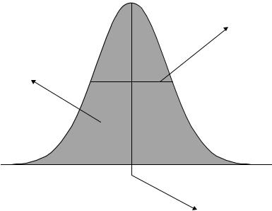
Peaks can be characterised in a number of ways, but a common approach, as illustrated in Figure 3.1, is to characterise each peak by

Width at half height

Area

Position of centre

Figure 3.1

Main parameters that characterise a peak

SIGNAL PROCESSING	123

1.a position at the centre (e.g. the elution time or spectral frequency),

2.a width, normally at half-height, and

3.an area.

The relationship between area and peak height is dependent on the peakshape, as discussed below, although heights are often easier to measure experimentally. If all peaks have the same shape, then the ratios of heights are proportional to ratios of areas. However, area is usually a better measure of chemical properties such as concentration and it is important to obtain precise information relating to peakshapes before relying on heights, for example as raw data for pattern recognition programs.

Sometimes the width at a different percentage of the peak height is cited rather than the half-width. A further common measure is when the peak has decayed to a small percentage of the overall height (for example 1 %), which is often taken as the total width of the peak, or alternatively has decayed to a size that relates to the noise.

In many cases of spectroscopy, peakshapes can be very precisely predicted, for example from quantum mechanics, such as in NMR or visible spectroscopy. In other situations, the peakshape is dependent on complex physical processes, for example in chromatography, and can only be modelled empirically. In the latter situation it is not always practicable to obtain an exact model, and a number of closely similar empirical estimates will give equally useful information.

Three common peakshapes cover most situations. If these general peakshapes are not suitable for a particular purpose, it is probably best to consult specialised literature on the particular measurement technique.

3.2.1.1 Gaussians

These peakshapes are common in most types of chromatography and spectroscopy. A simplified equation for a Gaussian is

xi = A exp[−(xi − x0)2/s2]

where A is the height at the centre, x0 is the position of the centre and s relates to the peak width.

Gaussians are based on a normal√ distribution where x0 corresponds to the mean of a series of measurements and s/ 2 to the standard deviation.

It can be shown that the width at half-height of a Gaussian peak is given by = √ √ 1/2

2s ln 2 and the area by π As using the equation presented above; note that this depends on both the height and the width.

Note that Gaussians are also the statistical basis of the normal distribution (see Appendix A.3.2), but the equation is normally scaled so that the area under the curve equals one. For signal analysis, we will use this simplified expression.

3.2.1.2 Lorentzians

The Lorentzian peakshape corresponds to a statistical function called the Cauchy distribution. It is less common but often arises in certain types of spectroscopy such as NMR. A simplified equation for a Lorentzian is

xi = A/[1 + (xi − x0)2/s2]

124	CHEMOMETRICS

Lorentzian

Gaussian

Figure 3.2

Gaussian and Lorentzian peakshapes of equal half-heights

where A is the height at the centre, x0 is the position of the centre and s relates to the peak width.

It can be shown that the width at half-height of a Lorentzian peak is given by1/2 = 2s and the area by π As; note this depends on both the height and the width.

The main difference between Gaussian and Lorentzian peakshapes is that the latter has a bigger tail, as illustrated in Figure 3.2 for two peaks with identical half-widths and heights.

3.2.1.3 Asymmetric Peakshapes

In many forms of chromatography it is hard to obtain symmetrical peakshapes. Although there are a number of sophisticated models available, a very simple first approximation is that of a Lorentzian/Gaussian peakshape. Figure 3.3(a) represents a tailing peakshape, in which the left-hand side is modelled by a Gaussian and the right-hand side by a Lorentzian. A fronting peak is illustrated in Figure 3.3(b); such peaks are much rarer.

3.2.1.4 Use of Peakshape Information

Peakshape information can be employed in two principal ways.

1.Curve fitting is fairly common. There are a variety of computational algorithms, most involving some type of least squares minimisation. If there are suspected (or known) to be three peaks in a cluster, of Gaussian shape, then nine parameters need to be found, namely the three peak positions, peak widths and peak heights. In any curve fitting it is important to determine whether there is certain knowledge of the peakshapes, and of certain features, for example the positions of each component. It is also important to appreciate that many chemical data are not of sufficient quality for very detailed models. In chromatography an empirical approach is normally adequate: over-modelling can be dangerous. The result of the curve fitting can be a better description of the system; for example, by knowing peak areas, it may be possible to determine relative concentrations of components in a mixture.

2.Simulations also have an important role in chemometrics. Such simulations are a way of trying to understand a system. If the result of a chemometric method

SIGNAL PROCESSING	125

(a)

(b)

Figure 3.3

Asymmetric peakshapes often described by a Gaussian/Lorentzian model. (a) Tailing: left is Gaussian and right Lorentzian. (b) Fronting: left is Lorentzian and right Gaussian

(such as multivariate curve resolution – see Chapter 6) results in reconstructions of peaks that are close to the real data, then the underlying peakshapes provide a good description. Simulations are also used to explore how well different techniques work, and under what circumstances they break down.

A typical chromatogram or spectrum consists of several peaks, at different positions, of different intensities and sometimes of different shapes. Figure 3.4 represents a cluster of three peaks, together with their total intensity. Whereas the right-hand side peak pair is easy to resolve visually, this is not true for the left-hand side peak pair, and it would be especially hard to identify the position and intensity of the first peak of the cluster without using some form of data analysis.

3.2.2 Digitisation

Almost all modern laboratory based data are now obtained via computers, and are acquired in a digitised rather than analogue form. It is always important to understand how digital resolution influences the ability to resolve peaks.

Many techniques for recording information result in only a small number of datapoints per peak. A typical NMR peak may be only a few hertz at half-width, especially using well resolved instrumentation. Yet a spectrum recorded at 500 MHz, where 8K (=8192) datapoints are used to represent 10 ppm (or 5000 Hz) involves each datapoint

126	CHEMOMETRICS

Figure 3.4

Three peaks forming a cluster

representing 1.64 = 8192/5000 Hz. A 2 Hz peakwidth is represented by only 3.28 datapoints. In chromatography a typical sampling rate is 2 s, yet peak half-widths may be 20 s or less, and interesting compounds separated by 30 s. Poor digital resolution can influence the ability to obtain information. It is useful to be able to determine how serious these errors are.

Consider a Gaussian peak, with a true width at half-height of 30 units, and a height of 1 unit. The theoretical area can be calculated using the equations in Section 3.2.1.1:

• the width at half-height is given by 2s

√

√

ln 2, so that s = 30/(2

ln 2) = 18.017 units;

•

=

=

the area is given by

√π As, but A

1, so that the area

is

√π 30/(2√ln 2)

31.934 units.

Typical units for area might be AU.s if the sampling time is in seconds and the intensity in absorption units.

Consider the effect of digitising this peak at different rates, as indicated in Table 3.1, and illustrated in Figure 3.5. An easy way of determining integrated intensities is simply to sum the product of the intensity at each datapoint (xi ) by the sampling interval (δ) over a sufficiently wide range, i.e. to calculate δ xi . The estimates are given in Table 3.1 and it can be seen that for the worst digitised peak (at 24 units, or once per half-height), the estimated integral is 31.721, an error of 0.67 %.

A feature of Table 3.1 is that the acquisition of data starts at exactly two datapoints in each case. In practice, the precise start of acquisition cannot easily be controlled and is often irreproducible, and it is easy to show that when poorly digitised, estimated integrals and apparent peakshapes will depend on this offset. In practice, the instrumental operator will notice a bigger variation in estimated integrals if the digital resolution is low. Although peakwidths must approach digital resolution for there to be significant errors in integration, in some techniques such as GC–MS or NMR this condition is often obtained. In many situations, instrumental software is used to smooth or interpolate the data, and many users are unaware that this step has automatically taken place. These simple algorithms can result in considerable further distortions in quantitative parameters.

SIGNAL PROCESSING	127

Time

0			20			40					60							80						100					120
Figure 3.5
Influence on the appearance of a peak as digital resolution is reduced
Table 3.1 Reducing digital resolution.
8 units								16 units										20 units											24 units
Time			Intensity					Time			Intensity						Time					Intensity						Time	Intensity
2			0.000			2					0.000						2	0.000						2					0.000
10			0.000			18					0.004						22	0.012						26					0.028
18			0.004			34					0.125						42	0.369						50					0.735
26			0.028			50					0.735						62	0.988						74					0.547
34			0.125			66					0.895						82	0.225						98					0.012
42			0.369			82					0.225						102	0.004
50			0.735			98					0.012
58			0.988			114					0.000
66			0.895
74			0.547
82			0.225
90			0.063
98			0.012
106			0.001
114			0.000
Integral			31.934								31.932							31.951											31.721

128	CHEMOMETRICS

A second factor that can influence quantitation is digital resolution in the intensity direction (or vertical scale in the graph). This is due to the analogue to digital converter (ADC) and sometimes can be experimentally corrected by changing the receiver gain. However, for most modern instrumentation this limitation is not so serious and, therefore, will not be discussed in detail below, but is illustrated in Problem 3.7.

3.2.3 Noise

Imposed on signals is noise. In basic statistics, the nature and origin of noise are often unknown, and assumed to obey a normal distribution. Indeed, many statistical tests such as the t-test and F -test (see Appendices A.3.3 and A.3.4) assume this, and are only approximations in the absence of experimental study of such noise distributions. In laboratory based chemistry, there are two fundamental sources of error in instrumental measurements.

1.The first involves sample preparation, for example dilution, weighing and extraction efficiency. We will not discuss these errors in this chapter, but many of the techniques of Chapter 2 have relevance.

2.The second is inherent to the measurement technique. No instrument is perfect, so the signal is imposed upon noise. The observed signal is given by

x = x˜ + e

where x˜ is the ‘perfect’ or true signal, and e is a noise function. The aim of most signal processing techniques is to obtain information on the true underlying signal in the absence of noise, i.e. to separate the signal from the noise. The ‘tilde’ notation is to be distinguished from the ‘hat’ notation, which refers to the estimated signal, often obtained from regression techniques including methods described in this chapter. Note that in this chapter, x will be used to denote the analytical signal or instrumental response, not y as in Chapter 2. This is so as to introduce a notation that is consistent with most of the open literature. Different investigators working in different areas of science often independently developed incompatible notation, and in a overview such as this text it is preferable to stick reasonably closely to the generally accepted conventions to avoid confusion.

There are two main types of measurement noise.

3.2.3.1 Stationary Noise

The noise at each successive point (normally in time) does not depend on the noise at the previous point. In turn, there are two major types of stationary noise.

1.Homoscedastic noise. This is the simplest to envisage. The features of the noise, normally the mean and standard deviation, remain constant over the entire data series. The most common type of noise is given by a normal distribution, with mean zero, and standard deviation dependent on the instrument used. In most real world situations, there are several sources of instrumental noise, but a combination of different symmetric noise distributions often tends towards a normal distribution. Hence this is a good approximation in the absence of more detailed knowledge of a system.

SIGNAL PROCESSING	129

2.Heteroscedastic noise. This type of noise is dependent on signal intensity, often proportional to intensity. The noise may still be represented by a normal distribution, but the standard deviation of that distribution is proportional to intensity. A form of heteroscedastic noise often appears to arise if the data are transformed prior to processing, a common method being a logarithmic transform used in many types of spectroscopy such as UV/vis or IR spectroscopy, from transmittance to absorbance. The true noise distribution is imposed upon the raw data, but the transformed information distorts this.

Figure 3.6 illustrates the effect of both types of noise on a typical signal. It is important to recognise that several detailed models of noise are possible, but in practice it is not easy or interesting to perform sufficient experiments to determine such distributions. Indeed, it may be necessary to acquire several hundred or thousand spectra to obtain an adequate noise model, which represents overkill in most real world situations. It is not possible to rely too heavily on published studies of noise distribution because each instrument is different and the experimental noise distribution is a balance between several sources, which differ in relative importance in each instrument. In fact, as the manufacturing process improves, certain types of noise are reduced in size and new effects come into play, hence a thorough study of noise distributions performed say 5 years ago is unlikely to be correct in detail on a more modern instrument.

In the absence of certain experimental knowledge, it is best to stick to a fairly straightforward distribution such as a normal distribution.

3.2.3.2 Correlated Noise

Sometimes, as a series is sampled, the level of noise in each sample depends on that of the previous sample. This is common in process control. For example, there may be problems in one aspect of the manufacturing procedure, an example being the proportion of an ingredient. If the proportion is in error by 0.5 % at 2 pm, does this provide an indication of the error at 2.30 pm?

Many such sources cannot be understood in great detail, but a generalised approach is that of autoregressive moving average (ARMA) noise.

Figure 3.6

Examples of noise. From the top: noise free, homoscedastic, heteroscedastic