Physics of biomolecules and cells

W. Bialek: Thinking About the Brain

513

itself does not add too much noise. But being quiet is not enough: to make maximally reliable estimates of nontrivial stimulus features like motion one must be sure to do the correct computation. To understand how this works let’s look at a simple example, and then I’ll outline what happens when we use the same formalism to look at motion estimation. My discussion here follows joint work with Marc Potters [54].

Suppose that someone draws a random number x from a probability distribution P (x). Rather than seeing x itself, you get to see only a noisy version, y = x + η, where η is drawn from a Gaussian distribution with variance σ2. Having seen y, your job is to estimate x, and for simplicity let’s say that the “best estimate” is best in the least squares sense, as above. Then from Problem 5 we know that the optimal estimator is the conditional mean,

xest(y) = dx xP (x|y).

Now we use Bayes’ rule and push things through:

xest(y) =

1

dx xP (y|x)P (x)

P (y)

1

1

1

=

√

dx xP (x) exp −

(y

− x)2

P (y)

2σ2

2πσ2

= Z(y)

dx x exp − kBTe

+ kBTe ,

1

Ve (x)

Fe x

(3.17)

(3.18)

(3.19)

(3.20)

where we can draw the analogy with statistical mechanics by noting the correspondences:

Ve (x)		x2
	= − ln P (x) +		(3.21)
kBTe		2σ2
kBTe = σ2			(3.22)
Fe = y.			(3.23)

Thus, making optimal estimates involves computing expectation values of position, the potential is (almost) the prior distribution, the noise level is the temperature, and the data act as an external force. The connection with statistical mechanics is more than a convenient analogy; it helps us in finding approximation schemes. Thus at large noise levels we are at high temperatures, and all other things being equal the force is e ectively small so we can compute the response to this force in perturbation theory. On the other hand, at low noise levels the computation of expectation values must be dominated by ground state or saddle point configurations.

514		Physics of Bio-Molecules and Cells
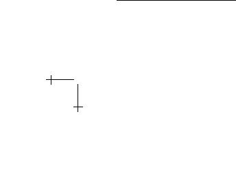
		Statistical mechanics	Optimal Estimation
		Temperature	Noise level
		Potential	(log) Prior distribution
		Average position	Estimate
		External force	Input data

In the case of visual motion estimation, the data are the voltages pro-

duced by the photoreceptors {Vn(t)} and the thing we are trying to estimate

is the angular velocity ˙( ). These are functions rather than numbers, but

θ t

this isn’t such a big deal if we are used to doing functional integrals. The

really new point is that ˙( ) does not directly determine the voltages. What

θ t

happens instead is that even if the fly flies along a perfectly straight path, so
˙	= 0, the world e ectively projects a movie C(x, t) onto the retina and
that θ

it is this movie which determines the voltages (up to noise). The motion θ(t) transforms this movie, and so enters in a strongly nonlinear way; if we take a one dimensional approximation we might write C(x, t) → C(x − θ(t), t). Each photodetector responds to the contrast as seen through an aperture function M (x − xn) centered on a lattice point xn in the retina, and for simplicity let’s take the noise to be dominated by photon shot noise. Since we have independent knowledge of the C(x, t), to describe the relationship

between ˙( ) and { ( )} we have to integrate over all possible movies,

θ t Vn t

weighted by their probability of occurrence P [C].

Putting all of these things together with our general scheme for finding

optimal estimates, we have
θ˙est(t0) =	Dθ θ˙(t0)P [θ(t)|{Vn (t)}]					1		(3.24)
P [θ(t)|{Vn (t)}] = P [{Vn(t)}|θ(t)]P [θ(t)]								(3.25)
				P [{Vn (t)}]
P [{Vn(t)}|θ(t)]	DC P [C] exp − 2			n		dt |Vn (t) − V¯n (t)|2
		R
V¯n(t) =								(3.26)
	dxM (x − xn)C(x − θ(t), t).							(3.27)

Of course we can’t do these integrals exactly, but we can look for approximations, and again we can do perturbation theory at low signal to noise levels and search for saddle points at high signal to noise ratios. When the

W. Bialek: Thinking About the Brain

515

dust settles we find [54]:

•At low signal to noise ratios the optimal estimator is quadratic in the receptor voltages,

θ˙est(t) ≈		dτ	dτ Vn (t − τ )Knm(τ, τ )Vm (t − τ ).	(3.28)

nm

•At moderate signal to noise ratios, terms with higher powers of the voltage become relevant and “self energy” terms provide corrections to the kernel Knm(τ, τ ).

•At high signal to noise ratios averaging over time becomes less important and the optimal estimator crosses over to

			˙
θ˙est(t)	≈		n Vn (t)[Vn (t) − Vn−1(t)]		2	,	(3.29)
				n[Vn (t) Vn−1(t)]
		constant +		−

where constant depends on the typical contrast and dynamics in the movies chosen from P [C(x, t)] and on the typical scale of angular velocities in P [θ(t)].

Before looking at the two limits in detail, note that the whole form of the motion computation depends on the statistical properties of the visual environment. Although the limits look very di erent, one can show that there is no phase transition and hence that increasing signal to noise ratio takes us smoothly from one limit to the other; although this is sort of a side point, it was a really nice piece of work by Marc. An obvious question is whether the fly is capable of doing these di erent computations under di erent conditions.

We can understand the low signal to noise ratio limit by realizing that when something moves there are correlations between what we see at the two space–time points (x, t) and (x + vτ, t + τ ). These correlations extend to very high orders, but as the background noise level increases the higher order correlations are corrupted first, until finally the only reliable thing left is the two–point function, and closer examination shows that near neighbor correlations are the most significant: we can be sure something is moving because signals in neighboring photodetectors are correlated with a slight delay. This form of “correlation based” motion computation was suggested long ago by Reichardt and Hassenstein based on behavioral experiments with beetles [55]; later work from Reichardt and coworkers explored the applicability of this model to fly behavior [42]. Once the motion sensitive neurons were discovered it was natural to check if their responses could be understood in these terms.

516	Physics of Bio-Molecules and Cells

There are two clear signatures of the correlation model. First, since the receptor voltage is linear in response to image contrast, the correlation model confounds contrast with velocity: all things being equal, doubling the image contrast causes our estimate of the velocity to increase by a factor of four (!). This is an observed property of the flight torque that flies generate in response to visual motion, at least at low contrasts, and the same quadratic behavior can be seen in the rate at which motion sensitive neurons generate spikes and even in human perception (at very low contrast). Although this might seem strange, it’s been known for decades. What is interesting here is that this seemingly disastrous confounding of signals occurs even in the optimal estimator: optimal estimation involves a tradeo between systematic and random errors, and at low signal to noise ratio this tradeo pushes us toward making larger systematic errors, apparently of a form made by real brains.

The second signature of correlation computation is that we can produce movies which have the right spatiotemporal correlations to generate

a nonzero estimate ˙est but don’t really have anything in them that we

θ

would describe as “moving” objects or features. Rob de Ruyter has a simple recipe for doing this [56], which is quite compelling (I recommend you try it yourself): make a spatiotemporal white noise movie ψ(x, t),

		, t )		= δ(x	−	x )δ(t	−	t ),	(3.30)
ψ(x, t)ψ(x

and then add the movie to itself with a weight and an o set:

C(x, t) = ψ(x, t) + aψ(x + ∆x, t + ∆t).

(3.31)

Composed of pure noise, there is nothing really moving here. If you watch the movie, however, there is no question that you think it’s moving, and the fly’s neurons respond too (just like yours, presumably). Even more impressive is that if you change the sign of the weight a... the direction of motion reverses, as predicted from the correlation model.

Because the correlation model has a long history, it is hard to view evidence for this model as a success of optimal estimation theory. The theory of optimal estimation also predicts, however, that the kernel Knm(τ, τ ) should adapt to the statistics of the visual environment, and it does. Most dramatically one can just show random movies with di erent correlation times and then probe the transient response of H1 to step motions; the time course of transients (presumably reflecting the details of K) can vary over nearly two orders of magnitude from 30–300 msec in response to di erent correlation times [56]. All of this makes sense in light of optimal estimation theory but again perhaps is not a smoking gun. Closer to a real test is Rob’s argument that the absolute values of the time constants seen in such adaptation experiments match the frequencies at which natural movies would fall below

W. Bialek: Thinking About the Brain

517

SN R = 1 in each photoreceptor, so that filtering in the visual system is set (adaptively) to fit the statistics of signals and noise in the inputs [56, 57].

What about the high SNR limit? If we remember that voltages are linear in contrast, and let ourselves ignore the lattice in favor of a continuum limit, then the high SNR limit has a simple structure,

˙			dx (∂t C)(∂x C)				∂tC		(3.32)
θest(t)	≈				x	→		,
							x
		B +			dx (∂ C)2		∂ C

where the last limit is at high contrasts. As promised by the lack of a phase transition, this starts as a quadratic function of contrast just like the correlator, but saturates as the ratio of temporal and spatial derivatives. Note that if C(x, t) = C(x + vt), then this ratio recovers the velocity v exactly. This simple ratio computation is not optimal in general because real movies have dynamics other than rigid motion and real detectors have noise, but there is a limit in which it must be the right answer. Interestingly, the correlation model (with multiplicative nonlinearity) and the ratio of derivatives model (with a divisive nonlinearity) have been viewed as mutually exclusive models of how brains might compute motion. One of the really nice results of optimal estimation theory is to see these seemingly very di erent models emerge as di erent limits of a more general strategy. But, do flies know about this more general strategy?

The high SNR limit of optimal estimation predicts that the motion estimate (and hence, for example, the rate at which motion sensitive neurons generate spikes) should saturate as a function of contrast, but this contrast– saturated level should vary with velocity. Further, if one traces through the calculations in more detail, the the constant B and hence the contrast level required for (e.g.) half–saturation should depend on the typical contrast and light intensity in the environment. Finally, this dependence on the environment really is a response to the statistics of that environment, and hence the system must use some time and a little “memory” to keep track of these statistics–the contrast response function should reflect the statistics of movies in the recent past. All of these things are observed [56–58].

So, where are we? The fly’s visual system makes nearly optimal estimates of motion under at least some conditions that we can probe in the lab. The theory of optimal estimation predicts that the structure of the motion computation ought to have some surprising properties, and many of these are observed–some were observed only when theory said to go look for them, which always is better. I would like to get a clearer demonstration that the system really takes a ratio, and I think we’re close to doing that [59]. Meanwhile, one might worry that theoretical predictions depend too much on assumptions about the structure of the relevant probability distributions P [C] and P [θ], so Rob is doing experiments where he

518	Physics of Bio-Molecules and Cells

walks through the woods with both a camera and gyroscope mounted on his head (!), sampling the joint distribution of movies and motion trajectories. Armed with these samples one can do all of the relevant functional integrals by Monte Carlo, which really is lovely since now we are in the real natural distribution of signals. I am optimistic that all of this will soon converge on a complete picture. I also believe that the success so far is su cient to motivate a more general look at the problem of optimization as a design principle in neural computation.

4 Toward a general principle?

One attempt to formulate a general principle for neural computation goes back to the work of Attneave [60] and Barlow [61,62] in the 1950s. Focusing on the processing of sensory information, they suggested that an important goal of neural computation is to provide an e cient representation of the incoming data, where the intuitive notion of e ciency could be made precise using the ideas of information theory [63].

Imagine describing an image by giving the light intensity in each pixel. Alternatively, we could give a description in terms of objects and their locations. The latter description almost certainly is more e cient in a sense that can be formalized using information theory. The idea of Barlow and Attneave was to turn this around–perhaps by searching for maximally e cient representations of natural scenes we would be forced to discover and recognize the objects out of which our perceptions are constructed. E cient representation would have the added advantage of allowing the communication of information from one brain region to another (or from eye to brain along the optic nerve) with a minimal number of nerve fibers or even a minimal number of action potentials. How could we test these ideas?

•If we make a model for the class of computations that neurons can do, then we could try to find within this class the one computation that optimizes some information theoretic measure of performance. This should lead to predictions for what real neurons are doing at various stages of sensory processing;

•We could try to make a direct measurement of the e ciency with which neurons represent sensory information;

•Because e cient representations depend on the statistical structure of the signals we are trying to represent, a truly e cient brain would adapt its strategies to track changes in these statistics, and we could search for this “statistical adaptation”. Even better would be if we

W. Bialek: Thinking About the Brain	519
could show that the adaptation has the right form	to optimize
e ciency.

Before getting started on this program we need a little review of information theory itself16. Almost all statistical mechanics textbooks note that the entropy of a gas measures our lack of information about the microscopic state of the molecules, but often this connection is left a bit vague or qualitative. Shannon proved a theorem that makes the connection precise [63]: entropy is the unique measure of available information consistent with certain simple and plausible requirements. Further, entropy also answers the practical question of how much space we need to use in writing down a description of the signals or states that we observe.

Two friends, Max and Allan, are having a conversation. In the course of the conversation, Max asks Allan what he thinks of the headline story in this morning’s newspaper. We have the clear intuitive notion that Max will “gain information” by hearing the answer to his question, and we would like to quantify this intuition. Following Shannon’s reasoning, we begin by assuming that Max knows Allan very well. Allan speaks very proper English, being careful to follow the grammatical rules even in casual conversation. Since they have had many political discussions Max has a rather good idea about how Allan will react to the latest news. Thus Max can make a list of Allan’s possible responses to his question, and he can assign probabilities to each of the answers. From this list of possibilities and probabilities we can compute an entropy, and this is done in exactly the same way as we compute the entropy of a gas in statistical mechanics or thermodynamics: If the probability of the nth possible response is pn, then the entropy is

S = − pn log2 pn bits.	(4.1)

n

The entropy S measures Max’s uncertainty about what Allan will say in response to his question. Once Allan gives his answer, all this uncertainty is removed–one of the responses occurred, corresponding to p = 1, and all the others did not, corresponding to p = 0–so the entropy is reduced to zero. It is appealing to equate this reduction in our uncertainty with the information we gain by hearing Allan’s answer. Shannon proved that this is not just an interesting analogy; it is the only definition of information that conforms to some simple constraints.

16At Les Houches this review was accomplished largely by handing out notes based on courses given at MIT, Princeton and ICTP in 1998–99. In principle they will become part of a book to be published by Princeton University Press, tentatively titled Entropy, Information and the Brain. I include this here so that the presentation is self–contained, and apologize for the eventual self–plagiarism that may occur.

520	Physics of Bio-Molecules and Cells

To start, Shannon assumes that the information gained on hearing the answer can be written as a function of the probabilities pn17. Then if all N possible answers are equally likely the information gained should be a monotonically increasing function of N . The next constraint is that if our question consists of two parts, and if these two parts are entirely independent of one another, then we should be able to write the total information gained as the sum of the information gained in response to each of the two subquestions. Finally, more general multipart questions can be thought of as branching trees, where the answer to each successive part of the question provides some further refinement of the probabilities; in this case we should be able to write the total information gained as the weighted sum of the information gained at each branch point. Shannon proved that the only function of the {pn} consistent with these three postulates–monotonicity, independence, and branching–is the entropy S, up to a multiplicative constant.

If we phrase the problem of gaining information from hearing the answer to a question, then it is natural to think about a discrete set of possible answers. On the other hand, if we think about gaining information from the acoustic waveform that reaches our ears, then there is a continuum of possibilities. Naively, we are tempted to write

Scontinuum = − dxP (x) log2 P (x), (4.2)

or some multidimensional generalization. The di culty, of course, is that probability distributions for continuous variables [like P (x) in this equation] have units–the distribution of x has units inverse to the units of x–and we should be worried about taking logs of objects that have dimensions. Notice that if we wanted to compute a di erence in entropy between two distributions, this problem would go away. This is a hint that only entropy di erences are going to be important18.

17In particular, this “zeroth” assumption means that we must take seriously the notion of enumerating the possible answers. In this framework we cannot quantify the information that would be gained upon hearing a previously unimaginable answer to our question.

18The problem of defining the entropy for continuous variables is familiar in statistical mechanics. In the simple example of an ideal gas in a finite box, we know that the quantum version of the problem has a discrete set of states, so that we can compute the entropy of the gas as a sum over these states. In the limit that the box is large, sums can be approximated as integrals, and if the temperature is high we expect that quantum e ects are negligible and one might naively suppose that Planck’s constant should disappear from the results; we recall that this is not quite the case. Planck’s constant has units of momentum times position, and so is an elementary area for each pair of conjugate position and momentum variables in the classical phase space; in the classical limit the entropy becomes (roughly) the logarithm of the occupied volume in

W. Bialek: Thinking About the Brain

521

Returning to the conversation between Max and Allan, we assumed that Max would receive a complete answer to his question, and hence that all his uncertainty would be removed. This is an idealization, of course. The more natural description is that, for example, the world can take on many states W , and by observing data D we learn something but not everything about W . Before we make our observations, we know only that states of the world are chosen from some distribution P (W ), and this distribution has an entropy S(W ). Once we observe some particular datum D, our (hopefully improved) knowledge of W is described by the conditional distribution P (W |D), and this has an entropy S(W |D) that is smaller than S(W ) if we have reduced our uncertainty about the state of the world by virtue of our observations. We identify this reduction in entropy as the information that we have gained about W .

Problem 6: Maximally informative experiments. Imagine that we are trying to gain information about the correct theory T describing some set of phenomena. At some point, our relative confidence in one particular theory is very high; that is, P (T = T ) > F · P (T = T ) for some large F . On the other hand, there are many possible theories, so our absolute confidence in the theory T might nonetheless be quite low, P (T = T ) << 1. Suppose we follow the “scientific method” and design an experiment that has a yes or no answer, and this answer is perfectly correlated with the correctness of theory T , but uncorrelated with the correctness of any other possible theory–our experiment is designed specifically to test or falsify the currently most likely theory. What can you say about how much information you expect to gain from such a measurement? Suppose instead that you are completely irrational and design an experiment that is irrelevant to testing T but has the potential to eliminate many (perhaps half) of the alternatives. Which experiment is expected to be more informative? Although this is a gross cartoon of the scientific process, it is not such a terrible model of a game like “twenty questions”. It is interesting to ask whether people play such question games following strategies that might seem irrational but nonetheless serve to maximize information gain [64]. Related but distinct criteria for optimal experimental design have been developed in the statistical literature [65].

Perhaps this is the point to note that a single observation D is not, in fact, guaranteed to provide positive information, as emphasized by

phase space, but this volume is measured in units of Planck’s constant. If we had tried to start with a classical formulation (as did Boltzmann and Gibbs, of course) then we would find ourselves with the problems of equation (4.2), namely that we are trying to take the logarithm of a quantity with dimensions. If we measure phase space volumes in units of Planck’s constant, then all is well. The important point is that the problems with defining a purely classical entropy do not stop us from calculating entropy di erences, which are observable directly as heat flows, and we shall find a similar situation for the information content of continuous (“classical”) variables.

522	Physics of Bio-Molecules and Cells

DeWeese & Meister [66]. Consider, for instance, data which tell us that all of our previous measurements have larger error bars than we thought: clearly such data, at an intuitive level, reduce our knowledge about the world and should be associated with a negative information. Another way to say this is that some data points D will increase our uncertainty about state W of the world, and hence for these particular data the conditional distribution P (W |D) has a larger entropy than the prior distribution P (D). If we identify information with the reduction in entropy, ID = S(W ) −S(W |D), then such data points are associated unambiguously with negative information. On the other hand, we might hope that, on average, gathering data corresponds to gaining information: although single data points can increase our uncertainty, the average over all data points does not.

If we average over all possible data–weighted, of course, by their probability of occurrence P (D), we obtain the average information that D provides about W ,

I(D → W ) =					(4.3)
	S(W ) − P (D)S(W |D)
=	D	P (W )P (D)		·	(4.4)
	P (W, D) log2
			P (W, D)

W D

Note that the information which D provides about W is symmetric in D and W . This means that we can also view the state of the world as providing information about the data we will observe, and this information is, on average, the same as the data will provide about the state of the world. This “information provided” is therefore often called the mutual information, and this symmetry will be very important in subsequent discussions; to remind ourselves of this symmetry we write I(D; W ) rather than I(D → W ).

Problem 7: Positivity of information. Prove that the mutual information

I (D → W ), defined in equation (4.4), is positive.

One consequence of the symmetry or mutuality of information is that we can write

	(4.5)
I(D; W ) = S(W ) − P (D)S(W |D)
D
= S(D) − P (W )S(D|W ).	(4.6)

W

If we consider only discrete sets of possibilities then entropies are positive (or zero), so that these equations imply

I(D; W ) ≤ S(W )	(4.7)
I(D; W ) ≤ S(D).	(4.8)