The Elisa guidebook

Fig. 8.

Population distributions. (A) Gaussian or "normal" distribution. This is symmetrical about the mean and the values of the mean, median, and mode are the same. (B) A long "tail" of higher values, this represents a nonsymmetrical distribution in which there are different values for the mean, median, and mode (C).

same way, 1.96 ¡Á SD on either side of the mean contains 95% of the entire population. The 99% limits fall 2.58 SDs to either side of the mean.

The methods involved in calculating the mean, median, mode, and SD are usually made through the use of a statistical package, and the theory of their calculation can be examined in any fundamental book on statistics.

The confidence in results is important in the examination of distributions. This is considered in the calculation of the distribution statistics per se, but generally the greater the number of samples analyzed to calculate a distribu-

Page 340

Fig. 9.

Probability distribution for a population defined by Guassian curve.

Mean , and plus or minus 1, 2, 3 ¡Á SD encompases the percentages indicated. Thus, e.g., 95% of all results in a population would be distributed about the mean between +2 and ¨C2 ¡Á SD.

tion, the greater the confidence one can have in evaluating any result with respect to that distribution. The confidence value for any sample can be measured and used to ascribe confidence in a result with regard to the distribution statistic, although this is not common.

6.2.2¡ª

Nonnormal Distributions

The analysis of nonnormal distributions requires more complex mathematical considerations. Differences among mean, median, and mode alert the operator to nonsymetrical distributions.

6.3¡ª

Variation in Practice

The mean , SD, and %CV are used as indicators of the variation on data. The formula for is as follows:

in which X is an individual component and N is the sample size.

The formula for SD and %CV are as follows:

Page 341

Worked examples of the use of statistics is most worthwhile.

6.3.1¡ª Example Data

A number of supposedly negative samples (n = 421) have been analyzed by an indirect ELISA for the detection of antibodies. A single dilution was measured for each sample and the data were collected as OD values and based on a validated assay. Note that one concept in validation is the examination of populations to establish what we think of as a negative result. The distribution of data from a selected "negative" population will help describe any other test result as falling into or out of that population. Whether the population is actually negative with respect, e.g., of detecting a specific antibody is important and not always easy to ascertain. Examination of a large data set will indicate possible problems in determining whether there is wider dispersion (range) of results than might be expected. What is expected in a negative population is that all results will be low (OD) with a low variation. This can be examined, and any results with very high ODs can be reexamined. The object here is to plot the data as a frequency distribution and then calculate the mean and SD of that population. The selection of a negative population is easier from countries where there has never been a particular disease, but this does not rule out nonspecific results nor that the parameters measured, say, in cattle from England are

the same as those in the Sudan.

6.3.1.1¡ª Data

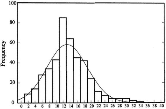
Figure 10 shows all the data plotted as a frequency distribution. Since we have taken a relatively large population, this might be reasonably expected to represent the distribution inherent in the whole population. However, the sample must be regarded with respect to the estimated total number of animals in a population and the possible geographical variations.

Note that the calculated mean, median, and mode are similar, indicating a normal distribution. We can therefore use statistics to set various limits as to values with respect to the mean and SD. Thus, from the data shown in Fig. 10, we see that the mean is 13.18 and that the SD is 5.76. Hence, 95% of all results lay between plus and minus 2 ¡Á SD of the mean. Therefore, the mean plus 2 ¡Á SD = 24.7, and the mean minus 2 ¡Á SD = 1.68. Any values outside the upper value of 24.7 would be more unusual in the population of negatives, and above 3 ¡Á SD very unusual. The population examined appeared to give results that were normally distributed. The mean value of this population and the SD can be used to determine the positivity of samples. The confidence we can have in any datum point (sample) can be determined with respect to the calculations based on the negative population examined. This requires the consideration of some statistical terms.

Page 342

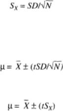
Fig. 10.

Distribution plot of 421 samples. Data were analyzed in a statistical program and showed the following: mean = 13.18; mode = 1 1.68; median = 12.00; lower quartile = 10; upper quartile = 16; interquartile range = 6; standard error of mean (SEM) - 0.28; variance = 33.20; SD = 5.76; CV = 0.44.

6.4¡ª

Confidence Interval

The CI for a mean essentially describes where the population mean (u) lies with respect to the sample

mean with a given probability. If several means are available from different groups of measurements of the same sample, the individual means will also be distributed normally around the grand mean. The random variation in a population of means is described by the SEM:

By using the SE of the experimentally determined mean one can give a CI that has a known probability of including the true population mean. This depends on the number of measurements (N), the SD and the level of confidence desired:

or

The value of t is taken from a table and depends on the level of confidence required or the level of probability (p) that u is outside the CI because of chance

Page 343

alone and the number of degrees of freedom (v, which is one less than the sample size) associated with the estimation of SD. Thus, values such as p = 0.05 indicate a 95% confidence limit [100 (1 ¨C p)%], that the interval includes the true mean. Basically, this means that we examine the variation in the result for a single sample (its mean and variation as error), and see where this fits in the distribution (with its internal variation).

The t values also fit a normal distribution. Here, one is making an assumption that the true population mean and SD are known, and because the CI is being made to include the true mean, the 0.5 probability that µ is beyond the calculated limits a is spread over both ends of the distribution (both tails). Here a two-sided interval, p = 0.5 t value, is used. The uses in which a single tail (above or below the mean) is considered, a one-sided t value (p = 0.025 is used (equivalent to the two-sided p = 0.05). The object then is (1) to have a defined total population statistic and (2) to examine where and with what confidence a sample value fits into this population. Some points need to be made concerning confidence limits.

1.No error can be calculated in which a single sample alone is measured. One element during the development of an assay is that the random error can be measured for many samples. This generally tends to be a compound of the internal variations of all aspects of sample analysis, and thus an overall generalized error can be calculated and "imposed" on all samples.

2.The SD of the population mean (SX) is smaller than the sample SD. The SD decreases as the square root of the number of samples is averaged; thus, obviously, the mean of the population is a better approximation of the true mean (u) than any single sample. As the number of samples increases, the CI for the mean increasingly decreases, because of the decreasing SD of the mean and of the decreasing value of t.

3.The defining of confidence limits requires the analyst to make a subjective choice of a level of confidence. The higher the level of confidence, the wider the limits.

As indicated already, the calculation of confidence limits does depend on the random errors following a Gaussian distribution, and this can be tested by χ2 squared or Kolmogorov-Smirnov testing, but in the main immunoassay, data follow the Gaussian statistic, which can often be proved throughout assay validation through repeat testing of samples.

7¡ª

Optimization of ELISA Procedures: New Approach

Recently, a method for optimizing ELISA procedures has been demonstrated (13). This method attempts to compare the net effects of different conditions using an experimental design called the Taguchi method. The method attempts to reduce the effects of the interactions of optimized variables, making it possible to access the optimal conditions even in cases in which there are large

Page 344

interactions among variables. The proposed scheme is said to allow calculation of the biochemical parameters of the ELISA. Thus, the calibration curve and the intra-and the interassay variability can be calculated in one step. This compares with the step-by-step approach of CBTs. The method is exemplified using an ELISA required to be optimal for the detection of the single-chain fragment of variable phages. The calculations are made through a spreadsheet program. This procedure is worth examining when considering the optimization of ELISAs and is one of the few designs intended to allow optimization based on a simple statistical evaluation. The design is based on that used to optimize the PCR (14,15).

References

1. Deshpande, S. S. (1996) in Enzyme Immunoassays from Concept to Product Development, Chapter 9, Chapman and Hall, International Thomson Publishing, New York.

2.Miller, J. J. and Valdes, R. (1991) Approaches to minimizing interference by cross-reactive molecules in immunoasays. Clin. Chem. 37, 144¨C153.

3.Westgard, J. O., Barry, P. L., and Hunt, M. R. (1981 ) A multi-rule Shewhart chart for quality control in clinical chemistry. Clin. Chem. 27, 493¨C501.

4.Blockx, P. and Martin, M. (1994) Laboratory quality assurance, in The Immunoassay Handbook (Wild, D., ed.), Stockton Press, New York, pp. 263¨C276.

5.Seth, J. (1991) Standardization and quality assurance, in Principles and Practice of Immunoassays (Price, C. P. and Newman, D. J., eds.), Stockton Press, New York, pp. 154¨C189.

6.Perlstein, M. T. (1987) Immunoassays. Quality control and troubleshooting, in Immunoassay: A practical Guide (Chan, D. W. and Perlstein, M. T., eds.), Academic, Orlando, FL, pp. 149¨C163.

7.Gosling, J. P. and Basso L. V. (1994). Quality assurance. in Immunoassay: Laboratory Analysis and Clinical Applications, (Gosling, J. P. and Basso, L. V., eds.), Butterworth-Heinemann, London, pp. 69¨C81.

8.Deshpand, S. S. (1996) Enzyme Immunoassays from Concept to Product Development. Chapman and Hall, International Thomson Publishing, New York.

9.Anderson, G. and Scott, M. (1991 ) Determination of product shelf life and activation energy required for five drugs of abuse. Clin. Chem. 37, 398¨C402.

10.Jacobson, R. H. (1998) Validation of serological assays for diagnosis of infectious diseases. Rev. Sci. Tech. OIE. 17, 469¨C486.

11.Office International des Epizooties (1998) Principles of validation of diagnostic assays for infectious diseases, in Manual of Standards for Diagnostic Tests and Vaccines, Office International des Epizooties (OIE), Paris, pp. 8¨C15.

12.Gardner, I. A. and Greiner, M. (1999) Advanced Methods for Test Validation and Interpretation in Veterinary Medicine. Freee University, Berlin and University of California, Davis, CA (report).

Page 345

13.Jeney, C., Dobay, O., Lengyel, A., Adam, E., and Nasz, I. (1999) Tagushi optimisation of ELISA procedures. J. Immunol. Methods 223, 137¨C146.

14.Cobb, B. B. and Clarkson, J. M. (1994) A simple procedure for optimizing the polymerase chain reaction (PCR) using modified Taguchi methods. Nucleic Acids Res. 18, 3801¨C3805.

15.Burch, G. J., Ferguson, C. H., Cartwright, G., and Kwong, F. Y. (1995) Application of Taguchi experimental design to the optimization of a baculo expression system. Biochem. Soc. Trans. 23(1), 107S.

Page 347

9¡ª

Charting Methods for Internal Quality Control

This chapter deals with relatively simple ways to use control charts to monitor the performance of ELISAs. A rinderpest competition ELISA, for the estimation of antibodies in serum samples, is used to demonstrate the methods. This assay is available in kit form. Constant evaluation of the use of the kit is part of what is called internal quality control (IQC). Figure 1 shows an overview of the ELISA scheme described in this chapter. The details of the procedure, which involves plotting the data graphically (charting methods), are explained herein. The objectives of charting data are as follows:

1.To keep a constant record of all data.

2.To monitor the assay from plate to plate in any one day's testing.

3.To monitor the tests made from day to day, week to week, year to year.

4.To allow rapid identification of unacceptable results.

5.To allow recognition of reagent problems.

6.To identify trends in results (increasingly poor performance).

7.To identify when a new set of kit reagents is necessary.

8.To allow identification of differences in operators of the assay.

9.To fulfill various criteria for good laboratory practice.

10.To fulfill necessary requirements for external recognition that tests are being performed at an acceptable level (increasingly important when results are used for international trading purposes).

1¡ª

Good Practice of IQC

IQC methods allow test operators as individuals to monitor the performance of their test. When there is more than one operator, the method produces a unification of approach, to allow control over results, and allows discrepancies among performance to be identified. It also promotes the idea of ''open" results that can be viewed by anyone, including outside scientists, interested in evaluating the status of a laboratory involved in providing results on which management decisions concerning disease control are made.

Page 348

Fig. 1.

Principles of competitive ELISA for measuring antibodies against rinderpest virus: (A) pretitration of indirect ELISA; (B) blocking of ELISA to detect antirinderpest antibodies in serum samples.

The method described here is not a deep statistical analysis of data. Rather, it attempts to visually assess results, so as to increase awareness of operators about what they are doing on a daily, monthly, and yearly cycle of work. The

Page 349

most important feature of testing in a laboratory is that operators have a very good understanding of the principles of the test they are using, and that they fully understand the nature of their test results and the need to process data. There is no substitute for this understanding, but the charting method recommended is an aid to simplifying the process of monitoring test performance. At first glance, this approach may seem to be overcomplicated. However, it is to be assumed that people involved in testing have had some trained and are running the assays on a fairly routine basis.

1.1¡ª

Principles of ELISA for Detection of Antibodies against Rinderpest

Figure 1 shows the principles of the ELISA used. The basis of the test is the prevention of pretitrated monoclonal antibody (mAb) from binding to rinderpest antigen on the wells of a microtiter plate by polyclonal antibodies in samples (serum). The degree of prevention is measured with reference to controls with no sample added (Cm) in which maximum optical density (OD) values are observed, and to wells in which is only conjugate is added (Cc) where low color is observed. Percentage inhibition (PI%) values are calculated with reference to these values.

Control serum samples are provided in the kits, which give strong (C++) and moderate (C+) PI% values. These controls can be used for assessment of the test from plate to plate and day to day. The plate design for the kits is shown in Fig. 2. For each plate, 40 samples are examined in duplicate, at a single dilution, and controls are placed as shown. Each PI% value is calculated with reference to the controls of individual plates. Studies on large numbers of negative sera and experimentally infected animals have determined the PI% values that ascribe positivity to samples.

On receipt of kits, operators should have everything to be able to perform the assay. The control sera enable operators to monitor the assay routinely, and the use of these data in control charts is the basis of this chapter. The necessary data for plotting on various charts is obtained through the calculation of the mean and standard deviation (SD), from the mean of control samples as raw OD data or PI% values.

2¡ª Charts

Two kinds of charts are recommended: (1) Daily Detailed Data (DDD) charts, used to plot data from single plates; and (2) Summary Data Charts (SDC), used to plot data from all plates performed on any day.

The use of such charts at various points of the rinderpest ELISA is illustrated in Fig. 3. The processing of data for plotting on the charts is important, and illustrative tables suitable for this purpose are presented in Figs. 4¨C7. Raw

Page 350