The Elisa guidebook

4.4¡ª

Example of Data

Table 6 gives typical results. The results obtained in your specific assay can be processed in the same way. Figure 17 is a diagrammatic representation of a stopped plate.

Since duplicates have been made, examine the variation between the values. This should not be high; that is, there should be little difference between the

Page 184

								Fig. 16.
				Micronics system for dilution of samples, showing the order of samples.
Table 6
Plate Data for Example Assaya
	1	2	3	4	5	6	7	8	9	10	11	12
A	1.21	1.09	0.78	0.32	0.12	0.66	0.65	0.17	0.67	0.34	1.34	1.11
B	1.19	1.03	0.69	0.31	0.16	0.64	0.62	0.16	0.64	0.37	1.28	1.17
C	1.00	0.23	0.45	0.56	0.78	0.13	0.19	0.45	0.56	0.78	1.00	0.56
D	0.97	0.27	0.49	0.54	0.72	0.16	0.20	0.44	0.53	0.75	1.01	0.55
E	0.13	0.14	0.18	0.09	0.07	0.12	0.14	0.09	0.08	0.12	0.16	0.14
F	0.12	0.13	0.16	0.09	0.08	0.11	0.13	0.10	0.09	0.11	0.13	0.15
G	0.15	0.18	0.13	0.14	0.10	0.15	0.13	0.12	0.13	0.13	0.12	0.08
H	0.13	0.16	0.13	0.15	0.12	0.13	0.12	0.14	0.15	0.12	0.11	0.09

aDuplicates of samples made are A1, B1; A2, B2; and so on. Suspect positive sera (24) are in rows A¨CD. Negative (prebleed sera) are in rows E¨CH.

ODs for both test wells of the same sample. Calculate the mean (average result) of the OD from both wells if the difference is not large. Variation in results are discussed later. Take the mean value to two decimal places.

4.5.1¡ª

Mean and Standard Deviation from Mean of Negative Serum Data

Take all the means of the negative sera and calculate the mean and standard deviation (SD) of the negative population using the calculator. (Note: Instruction should be given on the use of a calculator.) Noncourse users of the manual

Page 185

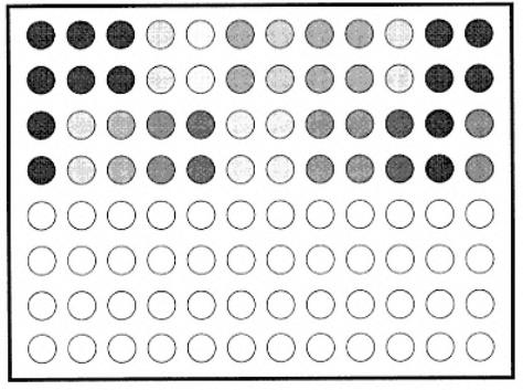
Fig. 17.

Diagrammatic representation of a stopped plate.

should obtain a calculator and follow operating instructions to calculate the same parameters.

4.5.2¡ª

Frequency Plots of Negative Serum OD Results

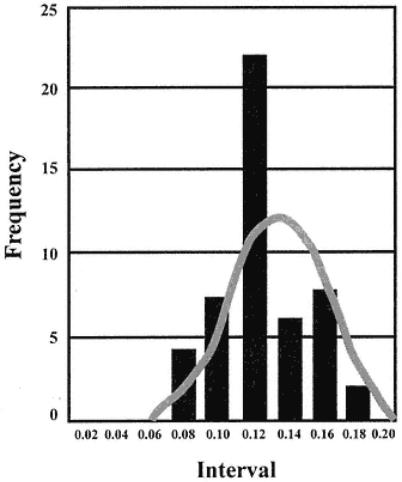
Plot the results for the negative sera as shown in Fig. 18. These relate the number of samples giving a particular OD.

A frequency distribution is obtained so that the distribution of negative results is obtained. Create a table of OD intervals and score the numbers of sera falling into the intervals. Add up the score, and plot this against the intervals. The mean of the data for the negative sera and the SD of the data can be found using a calculator. Thus, the population mean of a limited (in this case) negative population is found. If the population of negative ELISA readings is distributed normally (normal distribution statistics), then the upper limits of negativity can be ascribed with defined confidence limits depending on the number of SDs from the mean that is used.

The mean value in this case is 0.125, and the SD is 0.026. Thus, if we select 3X SD above this mean value (= 0.084) and add this to the mean value (= 0.209), any values equal to or above this value are unlikely to be part of the measured negative population as defined by the fact that only approx 0.1% of negative sera examined tended toward this value. Limits using 2X the SD above the measured negative population mean reduce confidence in the results for ascribing positivity (increase possible sensitivity but reduce specificity).

Page 186

Fig. 18.

Frequency plot relating number of sera giving particular

OD values. The gray curve is the normal distribution plot.

In practice, such distributions are skewed to the right-hand side, so that a tailing of results is seen at the higher ODs (see Fig. 19). To establish an OD reading that reflects the upper limit of negativity (since all negative sera have been studied), a statistical evaluation of the distribution is required. In general, since the distribution is skewed, a value of two times the mean OD for all the negative sera has been found to determine the upper limit of negativity (which corresponds to the lower limit of positivity) with a 95% confidence limit. Thus, we are 95% certain that a sample giving an OD value of equal to or greater than the value at two times the mean of the negative population OD results is positive. In practice, a confidence limit of 99% can be ascribed to results equal or greater than two times the population mean.

4.5.3¡ª Problems

When examining negative populations, we are assuming such sero-negativity using one or more factors, such as other serological test results, knowledge of the clinical history of the animals, and epidemiological factors. Thus, it may

Page 187

Fig. 19.

Distribution skewed to the right.

be easy to identify seronegative animals in countries where a particular disease has never been recorded. However, this may not be true for countries that have endemic disease or where vaccination campaigns have been mounted at various times (with variable amounts of antibody against specific disease agents being elicited). In such conditions, the experimenter might make the best assessment of likely negative animals. In this case, after plotting the frequency curves, one of several distributions might be obtained:

1.Figure 19: One peak at the low OD end of distribution. The population is probably negative with all sera showing low OD.

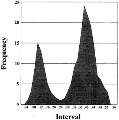
2.Figure 20: Two peaks fairly well separated at the low OD and at the higher OD end of distribution. Distinct populations of animals that are positive and negative may reflect recent infection or vaccination.

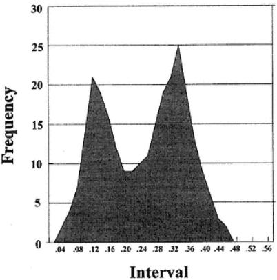
3.Figure 21: Twopeaks merged. There is no clear distinction between populations (the high and low ODs greatly overlap). These curves also illustrate what the picture looks like after sampling total populations containing positive and negative animals. Thus, for the example in Fig.19, there is no problem in ascribing an upper limit for negativity. Obviously the sera show the type of result expected of

Page 188

Fig. 20.

Frequency plot of OD results from analysis of sera, with two peaks representing distinct populations.

a totally negative population. However, in Fig. 20 we have a percentage of high OD results. These probably represent positive animals, and we can use the clear difference in the two distributions obtained to suggest strongly that the low OD results represent a negative population.

The distribution in Fig. 21 demonstrates a situation in which there is a heterogeneous population of animals with respect to their levels of antibodies. Thus, it is probable that the low OD range (which is shown by the situations in Figs. 19 and 20) represents negative animals. The merging of high and low results with high numbers of animals probably indicates that antibody levels have been reduced in the population after a past infection. Such a population can be studied using a defined negative population (maybe from another source), but the negative distribution cannot be assessed from study of this type of distribution alone. Hence, the experimenter might obtain serum samples from relevant species from countries where the disease they wish to study is absent. The negative value(s) obtained from such sera may not always be the same as that of the indigenous stock, but for most exercises will suffice.

Page 189

Fig. 21.

Frequency plot of OD results from analysis of sera.

No clear distinction is seen between populations.

4.6¡ª

Establishment of Control Negative Sera

It is possible to use a limited number of negative sera to act as controls in any assay of antibodies. This can only be realistically done if a distribution of many negative serum OD levels has been made (approx 100 minimum). Thus, a serum typifying the mean of the population of negative sera can be used. If this is included as a single dilution in the indirect ELISA, the OD values obtained may represent the mean value for the negative serum population. The upper limit of negativity can then be calculated by multiplying this value by 2 (since we know that this is a relevant value after studying the distribution). This approach is relevant when multichannel spectrophotometers are be used to read the color.

If assessment by eye is being used, control negative sera giving OD levels at the upper limit of negativity (around two times the mean) might be used. Color development in such assays should then be allowed until color is just detectable in the negative controls. The test should then be stopped. Therefore, any wells showing color more intense than the control wells would be positive for antibody.

Page 190

Fig. 22.

Plate layout for comparison of test sera with standard serum titration.

4.6.1¡ª

Data Analysis

You have calculated the mean OD of the negative population as well as the SD from the mean of the population. Now find a serum that characterizes the mean of the population. As well as one that characterizes the upper limit (two times the mean) of the population.

4.7¡ª

Relating Single Test Dilutions to Standard Positive Antiserum Curves

If a characterized antiserum is available, it may be used as a standard in the indirect ELISA. In this case, a fulldilution range of the serum is made and titrated under identical conditions to the single dilutions of the test sera. A typical plate format is shown in Fig. 22. At the end of the test, a standard curve relating the OD to the dilution of standard positive serum is constructed. The titers of the test samples can then be read from this curve so that a relative assessment of activity is obtained. This is demonstrated in Fig. 23. The standard serum may be given an arbitrary activity (units) so that results may be expressed in those units. Such control positive sera may be useful when standardization between laboratories is required.

Page 191

Fig. 23.

Use of standard serum titration curve to assess titers of test sera. OD values obtained from serum A and B are read from the titration curve of the standard serum (a and b).

4.8¡ª

Complications of Actual Disease

Studies on many systems have shown that false positive results are obtained in a low percentage of animals from a guaranteed noninfected population. It is difficult to determine why such reactions occur, but several reasons have been proposed, such as contamination of the serum with bacteria and fungi, dietary factors, and heating of the sera. The percentage can be of the order 1¨C2%, and they are easily read as very high ODs as compared to the majority of samples giving the typical negative distributions already discussed. This nonspecificity may be eliminated, e.g., by using different antigenic preparations. However, the number of likely false positive results should be taken into account when diagnosing disease on a herd basis. Thus, if we know that 2 animals in 100 show this response and we find that 20 animals in 100 show high responses, it

Page 192

is likely that disease is diagnosed. However, if only one to three animals ''positive," this finding could be owing to the identified nonspecific reactions.

5¡ª

Use of Antibodies on Solid Phase in Capture ELISA

This section examines sandwich ELISAs for measurement of antigens and antibodies.

5.1¡ª

Use of Capture ELISA to Detect and Titrate Antigen

5.1.1¡ª

Learning Principles

1.Optimizing the amount of capture antibody attached to the wells.

2.Optimizing amount of detecting antibody.

5.1.2¡ª

Reaction Scheme

I	= microplate wells (solid phase)
ABX	= capture antibody (species X) specific for Ag
Ag	= antigen
AbY	= detecting antibody (species Y) specific for Ag
AntiAb*E	= antispecies Y antibody linked to enzyme
S	= Substrate/color detection system
W	= washing step

+= addition and incubation of reactants

In this exercise, the capture antibody, the detecting antibody and the conjugate are used at optimal dilutions.

5.1.3¡ª

Basis of Assay

Antigens can do the following:

1.Attach poorly to plastics.

2.Be present in low quantity, e.g., in tissue culture fluids.

3.Be present as a low percentage of total protein in a "dirty" sample (e.g., in feces or epithelium samples).

4.Be unavailable for purification and concentration, since they are antigenically unstable when separated from other serum components.

In these cases, the indirect assay is unsuitable for handling the antigen, because it relies on the attachment of the antigen directly to the wells. The capture assay overcomes many of these problems, since the antigen is attached to the wells via specific antibodies. The test relies on the availability of two antisera from different species, so that the conjugate reacting with the second (detecting) antibody does not react with the capture antibody. It is also essential that the antigen have at least two antigenic sites so that antibody may bind

Page 193

to allow the sandwich (the antigen being the filling). Thus, when small antigens are being used (e.g., peptides), they may not react in such assays owing to their limited antigenic targets. The test offers an advantage over the indirect assay in the quantification of antigens, since direct attachment of proteins to wells is often nonlinear (i.e., is not proportional to the amount of protein in the sample). This is exaggerated if contaminating proteins are present with the antigen (e.g., serum components), because these compete for plastic sites in a nonlinear way. Because the capture antibody is specific, it binds antigen proportionally over a large range of protein concentrations. Thus, such assays give reproducible results when quantification is required. The assay is practically identical to the indirect assay except that an extra step (the capture antibody) is added. Thus, we have three parameters to optimize:

1.The capture antibody.

2.The detecting antibody.

3.The conjugate against the detecting antibody.

5.1.4¡ª Materials

1.Capture antibody (ABX): = sheep anti-guinea pig Ig (an IgG preparation at approx 5 mg/mL in PBS).

2.Ag: = guinea pig Ig at 1 mg/mL or as prepared by the worker.

3.Detection antibody (AbY): rabbit anti-guinea pig Ig serum (Ab).

4.Anti-AbY*E: sheep anti-rabbit conjugate (HRP).

5.Microplates.

6.Multichannel, single-channel, 10-mL and 1-mL pipets.

7.Carbonate/bicarbonate buffer, pH 9.6.

8.PBS 1% BSA/Tween-20 (0.05%).

9.Solution of OPD in citrate buffer.

10.Hydrogen peroxide 30% (w/v).

11.Washing solution.

12.1 M sulfuric acid in water.

13.Paper towels.