Advanced Wireless Networks - 4G Technologies

238 EFFECTIVE CAPACITY

8.1.1 Effective traffic source

To avoid UPC violation at the network access point, typically a shaper is applied at the source to force the cell stream to conform to the negotiated UPC, resulting in an effective traffic source. If the user can tolerate a larger shaping delay, a UPC descriptor with smaller network cost can be chosen for the connection. So, the problem of selecting the UPC values for a cell stream can be formulated as:

λs,Bs	c λp, λs, Bs and P(shaping) ≤ ε and λm ≤ λs ≤ λp	(8.9)
min

where parameters (λm, λp) are assumed to be known a priori or obtained through measurements. The cost function c( ) is an increasing function of each argument and represents the cost to the network of accepting a call characterized by the UPC values (λp, λs, Bs). The shaping probability P(shaping), which depends on the cell stream characteristics, represents the probability that an arbitrary arriving cell will be delayed by the shaper.

In the case of an idealized traffic characterization CS(ε), defined by Equation (8.2), the values of B(μ, ε) for λm < μ < λp are recorded, where B(μ, ε) is the minimum bucket size that ensures a shaping probability less than ε for a leaky bucket with rate μ.

Alternatively, from the approximate statistical characterization, we can obtain an estimate
˘				˘
B(Cs, μ, ε) for this minimum bucket size. Substituting B(Cs, μ, ε) in Equation (8.9), we
have
min		(	˘
	c[λp, λs,		)	] and λm ≤ λs ≤ λp	(8.9a)
λs			B(CS, λs, ε

8.1.2 Shaping probability

In a x/D/1 model of the (μ, B) leaky bucket shaper, an arriving cell is delayed (shaped) if and only if the number of customers seen in the fictitious queue is B or greater. Otherwise, the cell is transmitted immediately without delay. Suppose that the user wants to choose the UPC descriptor (λp, λs, Bs) such that the probability that an arbitrary cell will be shaped is less than ε. For a fixed leak rate μ, we would like to determine the minimum bucket size B(μ, ε) required to ensure a shaping probability less than ε. On should remember that the shaping probability is an upper bound for the violation probability, i.e., the probability that an arriving cell is nonconforming, in the corresponding UPC policer. Let na be a random variable representing the number in the fictitious queue observed by an arbitrary cell arrival. Suppose that the number of customers in the fictitious queue upon cell arrival is given by n = N , where N ≥ 1 is an integer. This means that the new customer sees N − 1 customers in the queue and one customer currently in service.

	Therefore, the waiting time in the		queue W for				this customer lies in			the range
[(N − 1)/μ, N/μ]. Also we can say,			if W	for	this		customer lies in this range, then
n	=	N at the arrival epoch. In other words n		=	N		(N	−	1)/μ < W < N	/μ so n	≥

N (N − 1)/μ < W .

Based on this we can write P(na ≥ B) = P[W > (B − 1)/μ]. So by using Equation (8.3), the shaping probability can be expressed as

P(shaping) = P(na ≥ B) ≈ a(μ)e−b(μ)(B−1)/μ

EFFECTIVE TRAFFIC SOURCE PARAMETERS	239
From this relation, for P(shaping) = ε we get
˘	(8.10)
B(Cs, μ, ε) = [μ/b(μ)] log[a(μ)/ε] + 1

8.1.3 Shaping delay

We can also specify the shaping constraint in terms of delay. Consider a cell stream passing through a leaky bucket traffic shaper with parameters (μ, B). Recall that the state counter n may be viewed as the number of customers in a fictitious x/D/1 queue. If W represents the waiting time in queue experienced by a given customer arriving in the fictitious queue served at rate μ, the actual delay experienced by the cell corresponding to the given fictitious customer can be expressed as

D = max[0, W − (B − 1)/μ)]

(8.11)

Using Equation (8.3) and W from Equation (8.11) we have

P(D > Dmax) ≈ a(μ)e−b(μ)Dmax e−b(μ)(B−1)/μ

E[D]	≈	[a(μ)/b(μ)]e−b(μ)(B−1)/μ	(8.12)

Setting the expected delay equal to the target mean delay ¯ gives B as

D

¯	¯	(8.13)
B(Cs, μ, D) = [μ/b(μ)] log[a(μ)/b(μ)D] + 1

which will be referred to as mean delay constraint curve.

The cost function c(λp, λs, Bs) represents the amount of resources that should be allocated to a cell characterized by the UPC parameters (λp, λs, Bs). For a source with deterministic periodic on–off sample paths and a random offset, the lengths of the on and off periods are given by

Ton = Bs/(λp − λs) and Toff = Bs/λs

(8.14)

Consider an on–off source model in which the source alternately transmits at rate r during an on-period and is silent during an off-period. The mean on-period and off period lengths are given by β−1 and α−1, respectively. For mathematical tractability, Erlang-k distribution for on and off periods is assumed.

The effective bandwidth of a source is defined as the minimum capacity required to serve the traffic source so as to achieve a specified steady-state cell loss probability εmux, where the multiplexer or switch buffer size is denoted by Bmux. Using the result from Kobayashi and Ren [9], the effective bandwidth for this source model can be obtained as

c(eff ) = rα/(α + β) + r2αβK /(α + β)3

(8.15)

where K = − log εmux/(2k Bmux). If we set the mean on and off periods as β−1 = Ton and α−1 = Toff, then by using Equation (8.14) in Equation (8.15), we have

c(eff ) = λs + λs(λp − λs)KBs/λp

(8.16)

Now, the following cost function for a UPC controlled source can be defined:

c(λp, λs, Bs) = min[λp, c(eff)] = min[λp, λs + λs λp − λs KBs/λp]

(8.17)

240 EFFECTIVE CAPACITY

The value for parameter K should be chosen such that c(λp, λs, Bs) approximates the bandwidth allocation of the network CAC policy. The limiting behavior of the cost function with respect to K is

c(λp, λs, Bs) → λs as K → 0 and c(λp, λs, Bs) → λp as K → ∞

Real-time UPC estimation is based on observations of the cell stream over a time period T . The procedure consists of the following steps: (1) estimate the mean and peak cell rates; (2) choose a set of candidate sustainable rates; (3) obtain the characterization of the stream; (4) for each candidate sustainable rate, compute the minimum bucket size required to meet a user constraint on shaping delay; and (5) choose the candidate rate that minimizes the cost function.

The peak and mean rates can be estimated from observations of the cell stream over a window of length T . The interval is subdivided into smaller subintervals of equal length Ts = T /M. For example, in experiments with MPEG video sequences described in Mark and Ramamurthy [5], Ts was set equal to the frame period of 33 ms. If n is the total number of cell arrivals during T and ni the number of cell arrivals in the ith subinterval, then the mean

ˆ
rate can be estimated as λm = n/ T . For some applications, the peak rate may be known
ˆ	≤ i ≤ M}.
a priori. Otherwise, the peak rate can be estimated by λp = max{ni/ Ts; 1

Candidate rates μ1, . . . , μN are chosen between the mean and peak rates. The simplest approach is to choose N and space the candidate rates at uniform spacing between the mean and peak rates. However, with a more judicious method of assignment, the set of candidate rates can be kept small, while still including rates close to the near-optimal sustainable

		ˆ
rates. Suppose that a prior estimate of the operating sustainable rate, λs, is available. In
ˆ	ˆ	ˆ
the absence of prior knowledge, one could assign λs = (λm + λp)/2. The candidate rate

μN is assigned equal to	ˆ	N c coarsely
	λs. The remaining rates are grouped into a set of

spaced rates and Nf finely spaced rates, with N = Nc + Nf + 1 and with Nf even. The

coarse rates					ˆ		ˆ
	μ1, . . . , μNc are assigned to be spaced uniformly over the interval (λs, λp)
˘			˘	˘
as μi = λm + i c, i = 1, . . . , Nc, where c is defined as c = (λp				− λm)/(Nc + 1).˘The
remaining N	ˆ		as follows: μ			λ
	in the neighborhood of λ	s			j+Nc =		s	+
	f fine rates are assigned ˘
j f , j = 1, . . . , Nf/2, and μ j+Nc = λs − ( j − Nf/2) f , j = Nf/2, . . . , Nf, where f								=

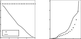
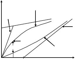
c/(Nc + 1). Figure 8.1 shows an example of the choice of candidate rates example with

N= 8, Nc = 3 and Nf = 4.

Measurement of traffic parameters is based on the bank of queues. The ith fictitious

queue is implemented using a counter ni that is decremented at the constant rate μi and incremented by 1 whenever a cell arrives [5]. For each rate μi , estimates of the queue

parameters (μi ) and ˆ(μi ) are obtained. Each queue is sampled at the arrival epoch of aˆ b

an ‘arbitrary’ cell. This sampling is carried out by skipping a random number of N j cells between the ( j-1)st and jth sampled arrivals. Since all of the fictitious queues are sampled at the same arrival epochs, only one random number needs to be generated for all queues at a sampling epoch. Over an interval of length T , a number of samples, say M, are taken from the queues. At the jth sampling epoch, the following quantities are recorded for each queue: Sj , the number of customers in service (so Sj {0, 1}); Q j , the number of customers in queue; and Tj , the remaining service time of the customer in service (if one is in service). After that the following sample means are computed:

M M M

aˆ = Sj /M; qˆ = Q j /M; τˆr = Tj /aˆ M

j=1 j=1 j=1

EFFECTIVE TRAFFIC SOURCE PARAMETERS

241

λp

		μ7		μ3
μ8	¯	μ6
	= λ s			μ2
		μ5
		μ4

λ m	Coarse rates:	μ1, μ2, μ3
	Fine rates:	μ	, μ	5	, μ	6	, μ
			4				7

Figure 8.1 Example of candidate rate assignment.

Parameter ˆ is then computed by using Equation (8.8) as b

where τˆr is approximated by

˘ C S =

ˆ	μaˆ		μaˆ
b = qˆ + μaˆ τˆr		≈ qˆ + aˆ /2

12 μ. The approximate statistical characterization is given by

ˆ ˆ	aˆ	ˆ
λp, λm		(μi ), b(μi ) : i = 1, . . . , N

Mapping to a UPC Descriptor is focused on the case where the user specifies a maximum

mean delay ¯ . The operating rate index is chosen to minimize the cost function defined in

D

Equation (8.17):

	i	*	= arg 1mini N	c	ˆ	ˆ	¯
					λp, μi , Bs	CS, μi , D
			≤ ≤
ˆ	¯
where Bs CS, μi , D is defined in Equation (8.13) and represents the bucket size required

¯
to achieve a mean delay of D at a leak rate μ. Then the operating UPC descriptor is assigned
as follows:
ˆ	ˆ	¯
λp = λp, λs = μi ,	Bs = Bs CS, μi , D

If the estimated mean and peak rates are close in value, the stream can be treated as a CBR stream. In this case, the UPC descriptor can simply be assigned according to the peak rate, i.e.

ˆ	Bs = 1
λp = λp, λs = μi ,

Some applications, such as video delivery, interactive multimedia sessions, etc., cannot be adequately characterized by a static set of parameters that are expected to hold for

242 EFFECTIVE CAPACITY

the entire session. The ability to renegotiate parameters during a session may be a viable way of efficiently supporting variable bit rate (VBR) traffic [5, 10] with real-time QoS constraints.

8.1.4 Performance example

In the MPEG standard for video compression, video is transmitted as a sequence of frames. For transmission over an ATM network, each MPEG frame must be segmented into ATM cells. In Mark and Ramamurthy [5], two modes of cell transmission over a frame interval are considered. In nonsmooth mode, the cells are transmitted at a constant rate λp starting at the beginning of the frame interval until the frame is fully transmitted. Then the source is silent until the beginning of the next frame interval. This results in an on–off type stream with correlated on and off periods. In smooth mode, the cells for the ith frame are transmitted at a constant rate f (i)/τ over the frame interval, where f (i) is the total number of cells in the i−th frame and τ is the interframe period. Thus, buffering is done to smooth out the transmission of cells of each frame over the corresponding frame interval.

Figure 8.2 shows the characterization ˆ S obtained empirically for an MPEG video stream

C

[5]. For this stream, the empirical mean and peak rates were determined to be 20 and 40.5 cells/ms, respectively. The two streams were offered to 19 queues running in parallel at the rates μ = 21, 22, . . . , 39 (cells/ms) and the corresponding values for [a(μ), b(μ)] were obtained according to the procedure described above. In the nonsmooth mode, a (μ) ≈ 1 for all values of μ while for smooth mode, a(μ) monotonically decreases as μ increases from λm to λp. On the other hand the b (μ) curves for the nonsmooth and smooth modes are close for μ near to the extremes λm and λp. For values of μ closer to the center of the interval (λm, λp), the curve for smooth mode lies above the curve for nonsmooth mode.

Thus, the characterization ˆ S captures the decrease in traffic burstiness due to intraframe

C

smoothing.

Figures 8.3 and 8.4 demonstrate that, for example, the shaping probability of 0.00001 at cell rate of 28 can be achieved with B = 1100 in the case of smooth mode while nonsmooth mode would require B = 2000 for the same shaping probability. More interesting results on this issue can be found in Mark and Ramamurthy [5].

1
0.8
0.6
a
0.4
0.2	non-smooth
	smooth
0
20	25	30	35	40

Rate (cells/ms)

	2000
	1500
b	1000
	500
	0
	20	25	30	35	40

Rate (cells/ms)

Figure 8.2 (a) a and (b) b parameters for MPEG.

EFFECTIVE LINK LAYER CAPACITY

243

	3500
							0.1
	3000						0.01
							0.001
(cells)	2500						0.0001
	2000
size
Bucket	1500
	1000
	500
	0
	20	22	24	26	28	30	32

Rate (cells/ms)

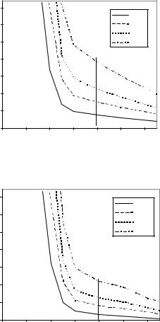
Figure 8.3 Shaping probability curves for nonsmooth mode.

	3500						0.1
	3000						0.01
							0.001
	2500						0.0001
B (cells)	2000
	1500
	1000
	500
	0
	20	22	24	26	28	30	32

Rate (cells/ms)

Figure 8.4 Shaping probability curves for smooth mode.

8.2 EFFECTIVE LINK LAYER CAPACITY

In the previous section we discussed the problem of effective characterization of the traffic source in terms of the parameters which are used to negotiate with the network a certain level of QoS. Similarly, on the network side, to enable the efficient support of quality of service (QoS) in 4G wireless networks, it is essential to model a wireless channel in terms of connection-level QoS metrics such as data rate, delay and delay-violation probability. The traditional wireless channel models, i.e. physical-layer channel models, do not explicitly characterize a wireless channel in terms of these QoS metrics. In this section, we discuss a link-layer channel model referred to as effective capacity (EC) [11]. In this approach, a wireless link is modeled by two EC functions, the probability of nonempty buffer and the QoS exponent of a connection. Then, a simple and efficient algorithm to estimate these EC functions is discussed. The advantage of the EC link-layer modeling and estimation is ease

244 EFFECTIVE CAPACITY

of translation into QoS guarantees, such as delay bounds and hence, efficiency in admission control and resource reservation.

Conventional channel models, discussed in Chapter 3, directly characterize the fluctuations in the amplitude of a radio signal. These models will be referred to as physical-layer channel models, to distinguish them from the link-layer channel model discussed in this section. Physical-layer channel models provide a quick estimate of the physical-layer performance of wireless communications systems (e.g. symbol error rate vs SNR). However, physical-layer channel models cannot be easily translated into complex link-layer QoS guarantees for a connection, such as bounds on delay. The reason is that these complex QoS requirements need an analysis of the queueing behavior of the connection, which cannot be extracted from physical-layer models. Thus, it is hard to use physical-layer models in QoS support mechanisms, such as admission control and resource reservation.

For these reasons, it was proposed to move the channel model up the protocol stack from the physical layer to the link layer. The resulting model is referred to as EC link model because it captures a generalized link-level capacity notion of the fading channel. Figure 8.5 illustrates the difference between the conventional physical-layer and link-layer model. For simplicity, the ‘physical-layer channel’ will be called the ‘physical channel’ and ‘link-layer channel’ will be referred to as the ‘link’.

8.2.1 Link-layer channel model

4G wireless systems will need to handle increasingly diverse multimedia traffic, which are expected to be primarily packet-switched. The key difference between circuit switching and packet switching, from a link-layer design viewpoint, is that packet switching requires queueing analysis of the link. Thus, it becomes important to characterize the effect of the data traffic pattern, as well as the channel behavior, on the performance of the communication system.

QoS guarantees have been heavily researched in the wired networks [e.g. ATM and Internet protocol (IP) networks]. These guarantees rely on the queueing model shown in

Instantaneous channel capacity log(1 + SNR)

Data

Network

Channel

Received SNR

access

Demodulator

sink

decoder

device

Receiver

Link-layer

Wireless

channel

channel

Data

Channel

Modulator

source

encoder

Network

access device

Physical-layer

Transmitter

channel

Figure 8.5 Packet-based wireless communication system.

	EFFECTIVE LINK LAYER CAPACITY		245
		Rate μ
	Data
	source	A(t)
		B
		Queue
		Q(t)
		Capacity
Channel		S(t)

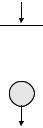
Figure 8.6 Queueing system model.

Figure 8.6 and studied in Chapter 6. This figure shows that the source traffic and the network service are matched using a first-in first-out buffer (queue). Thus, the queue prevents loss of packets that could occur when the source rate is more than the service rate, at the expense of increasing the delay. Queueing analysis, which is needed to design appropriate admission control and resource reservation algorithms, requires source traffic characterization and service characterization. The most widely used approach for traffic characterization is to require that the amount of data (i.e. bits as a function of time t) produced by a source conform to an upper bound, called the traffic envelope, (t). The service characterization for guaranteed service is a guarantee of a minimum service (i.e. bits communicated as a function of time) level, specified by a service curve SC (t)[12]. Functions (t) and (t) are specified in terms of certain traffic and service parameters, respectively. Examples include the UPC parameters, discussed in the previous section, used in ATM for traffic characterization, and the traffic specification (T-SPEC) and the service specification (R-SPEC) fields used with the resource reservation protocol [12] in IP networks.

A traffic envelope (t) characterizes the source behavior in the following manner: over any window of size t, the amount of actual source traffic A(t) does not exceed (t) (see Figure 8.7). For example, the UPC parameters, discussed in Section 8.1, specifies (t) by

(t) = min λp(s)t, λs(s)t + σ (s)

(8.18)

where λ(ps) is the peak data rate, λ(ss) the sustainable rate, and σ (s) = Bs the leaky-bucket size [12]. As shown in Figure 8.7, the curve (t) consists of two segments: the first segment has a slope equal to the peak source data rate λ(ps), while the second has a slope equal to the sustainable rate λ(ss), with λ(ss) < λ(ps). σ (s) is the y-axis intercept of the second segment.(t) has the property that A(t) ≤ (t) for any time t. Just as (t) upper bounds the source traffic, a network SC (t) lower bounds the actual service S(t) that a source will receive.

(t) has the property that (t) ≤ S(t) for any time t. Both (t) and (t) are negotiated during the admission control and resource reservation phase. An example of a network SC is the R-SPEC curve used for guaranteed service in IP networks

(t) = max λs(c)(t − σ (c)), 0 = λs(c)(t − σ (c)) +

(8.19)

where λ(sc) is the constant service rate, and σ (c) the delay (due to propagation delay, link sharing, and so on). This curve is illustrated in Figure 8.7. (t) consists of two segments;

σ (c)

σ (c)

246 EFFECTIVE CAPACITY

of bits
Number	Γ(t)
s(s)

lp(S )

Q(t)

t

Actual source traffic

A(t)

ls(s)

Ψ(t)

ls(c)

D(t)

Actual channel service

S (t)

t

s(c)

Time

Figure 8.7 Traffic and service characterization. (Reproduced by permission of IEEE [11].)

the horizontal segment indicates that no packet is being serviced due to propagation delay, etc., for a time interval equal to the delay σ (c), while the second segment has a slope equal to the service rate λ(sc). In the figure, the horizontal difference between A(t) and S(t), denoted D(τ ), is the delay experienced by a packet arriving at time τ , and the vertical difference between the two curves, denoted by Q(τ ), is the queue length built up at time τ , due to packets that have not been served yet.

As discussed in Chapter 4, providing QoS guarantees over wireless channels requires accurate models of their time-varying capacity, and effective utilization of these models for QoS support. The simplicity of the SCs discussed earlier motivates us to define the time-varying capacity of a wireless channel as in Equation (8.19). Specifically, we hope to lower bound the channel service using two parameters: the channel sustainable rate λ(sc), and the maximum fade duration σ (c).

Parameters λ(sc) and σ (c) are meant to be in a statistical sense. The maximum fade duration is a parameter that relates the delay constraint to the channel service. It determines the probability supt Pr{S(t) < (t)}. We will see later that σ (c) is specified by the source with

= Dmax, where D is the delay bound required by the source.

However, physical-layer wireless channel models do not explicitly characterize the channel in terms of such link-layer QoS metrics as data rate, delay and delay-violation probability. For this reason, we are forced to look for alternative channel models.

A problem that surfaces is that a wireless channel has a capacity that varies randomly with time. Thus, an attempt to provide a strict lower bound [i.e. the deterministic SC (t), used in IP networks] will most likely result in extremely conservative guarantees. For example, in a Rayleigh or Ricean fading channel, the only lower bound that can be deterministically guaranteed is a capacity of zero. The capacity here is meant to be delay-limited capacity, which is the maximum rate achievable with a prescribed delay bound (see Hanly and Tse [13] for details). This conservative guarantee is clearly useless in practice. Therefore, the

concept of deterministic SC	(t) is extended to a statistical version, specified as the pair
{ (t), ε}. The statistical SC {	(t), ε} specifies that the service provided by the channel,
˜	˜	(t) ≤ ε. In other words,
denoted S(t), will always satisfy the property that supt Pr S(t) <

ε is the probability that the wireless channel will not be able to support the pledged SC

EFFECTIVE LINK LAYER CAPACITY

247

(t), referred to as the outage probability. For most practical values of ε, a nonzero SC (t) can be guaranteed.

8.2.2 Effective capacity model of wireless channels

From the previous discussion we can see that for the QoS control we need to calculate an SC (t) such that, for a given ε > 0, the following probability bound on the channel service

˜ ( ) is satisfied:

S t

supt	˜	(t) ≤ ε and (t) =	(c)	(t − σ	(c)		+
	Pr S(t) <		λs			)		(8.20)

The statistical SC specification requires that we relate its parameters {λ(sc), σ (c), ε} to the fading wireless channel, which at the first sight seems to be a hard problem. At this point, the idea that the SC (t) is a dual of the traffic envelope (t) is used [11]. A number of papers exist on the so-called theory of effective bandwidth [14], which models the statistical behavior of traffic. In particular, the theory shows that the relation supt Pr {Q(t) ≥ B} ≤ ε is satisfied for large B, by choosing two parameters (which are functions of the channel rate r) that depend on the actual data traffic, namely, the probability of nonempty buffer, and the effective bandwidth of the source. Thus, a source model defined by these two functions fully characterizes the source from a QoS viewpoint. The duality between Equation (8.20) and supt Pr{Q(t) ≥ B} ≤ ε indicates that it may be possible to adapt the theory of effective bandwidth to SC characterization. This adaptation will point to a new channel model, which will be referred to as the effective capacity (EC) link model. Thus, the EC link model can be thought of as the dual of the effective bandwidth source model, which is commonly used in networking.

8.2.2.1 Effective bandwidth

The stochastic behavior of a source traffic can be modeled asymptotically by its effective bandwidth. Consider an arrival process { A(t), t ≥ 0}, where A(t) represents the amount of source data (in bits) over the time interval [0, t). Assume that the asymptotic log-moment generating function of A(t), defined as

(u) = tlim	1		log E eu A(t)	(8.21)
		t
→∞

exists for all u ≥ 0. Then, the effective bandwidth function of A(t) is defined as [11, 14]

α(u) =	(u)	u ≥ 0.	(8.22)
	u ,

This becomes more evident if we assume the constant traffic A(t) = A so that Equation (8.21) gives

(u) = tlim	1	log E eu A(t)	= tlim	1		log E eu A	= tlim	u A	= u tlim	A	= uα(u)
	t			t				t		t
→∞			→∞				→∞		→∞		(8.21a)

Consider now a queue of infinite buffer size served by a channel of constant service rate r, such as an AWGN channel. Owing to the possible mismatch between A(t) and S(t), the