C H A L L E N G E S F O R T H E E C O N O M I C S Y S T E M

295

P	LRAS
	AD2	SRAS
	AD1
P*		recessionary gap
	SRY*	Y
		Y*

F I G U R E 8 . 5 C L O S I N G T H E R E C E S S I O N A R Y G A P : K E Y N E S I A N A P P R O A C H

close the recessionary gap. This implies a shift of the aggregate demand function. For example, if the government increases its expenditure it can, through the multiplier, close the gap as shown in Figure 8.5.

Aggregate demand rises from AD1 to AD2 as the government increases its expenditure or cuts taxes via its discretionary fiscal policy. Moving from the shortrun equilibrium of P and SRY (from the intersection of SRAS and AD1) to the long-run equilibrium of P and Y we see that the boost in aggregate demand gives rise to a higher output level at the same aggregate level of prices.

8.2.4THE COSTS OF UNEMPLOYMENT

At the level of the macroeconomy, unemployed resources mean unproductive resources. Output is less than what it could be and income is below its potential level (at SRY relative to Y ). Economic activity is lower than if the economy operated at its full employment level. Some unemployment – a natural rate – is normal for any economy but non-voluntary unemployment generates costs. As well as reduced output and income, unemployment reduces governments’ revenue from tax income. With high employment, there is likely to be high demand for goods and services from firms. Firms may even make higher profits as consumers are able to buy more goods and services, but this depends on market structure, which we saw in Chapter 6. With high unemployment, profits surely suffer as demand is weakened.

Within modern welfare states, governments provide transfer payments as benefits to the unemployed (under certain conditions) and therefore, this represents an additional cost. Managing to create jobs for the unemployed would therefore increase national output, allow workers to earn a wage/salary, allow firms to make

296	T H E E C O N O M I C S Y S T E M

profits, allow the government to collect more in taxes and, if demand for labour were substantial, allow those already employed to increase their supply of labour.

All of the costs described above are at the level of the macroeconomy. Arguably, there are even more serious costs of unemployment if we consider the microeconomic, individual and social costs of unemployment. Even short-term unemployment can be disheartening and stressful for individuals and their families. This may result in higher personal costs for physical and mental health care, which can result from stress. Some authors have associated crime and delinquency with unemployment. In addition, individuals’ human capital can decline. A broad assessment of the costs of unemployment would take these issues into account also.

8 . 3 I N F L A T I O N

In Chapter 5 an example was used to illustrate how inflation is measured using information on people’s general expenditure patterns and the prices of goods and services. It is possible to consider the causes of inflation using the aggregate demand and supply model to examine what happens to the equilibrium price level if there are changes to either the demand or supply sides of the aggregate economy.

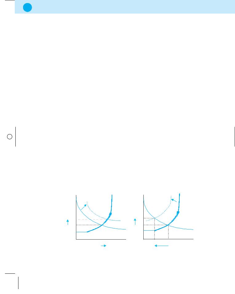
In Figure 8.6, beginning with panel A, we see a rise in aggregate demand, i.e. the AD curve shifting to the right from AD to AD1. The initial equilibrium occurs at

P and Y while the new equilibrium arises at P1 and Q1. An increase in aggregate demand leads to both higher output for the economy and a higher aggregate price level as the economy was not initially operating at potential output.

A: Demand pull
P	AS
AD
P1
P*	AD1
	Y
	Y* Y1

B: Cost push
P	AD	AS1	AS
P1
P*
	Y1	Y*	Y

F I G U R E 8 . 6 D E M A N D - P U L L A N D C O S T - P U S H I N F L A T I O N

C H A L L E N G E S F O R T H E E C O N O M I C S Y S T E M

297

An increase in the price level of an economy caused by rising aggregate demand is called demand-pull inflation.

Demand-pull inflation is associated with boom periods in an economy where planned expenditures rise with the increasing income generated in a boom. This means the aggregate demand curve moves up or rightwards on a continual basis over a period of time. Firms react to the increases in planned expenditures by producing more, if they can, and by raising prices.

If an economy is operating at capacity where all firms are producing to capacity, or beyond its long-run level, which can occur for short periods if workers are willing to work overtime, any rise in aggregate demand leads to increases in prices only and no increase in output.

An alternative source of inflation is presented in Figure 8.6 panel B where aggregate supply falls in response to firms’ reducing their output (in reaction to a rise in costs). For example, if firms’ wages increase then at any level of prices, firms would cut back on their production and this is observed in a leftward shift of aggregate supply.

Cost-push inflation occurs when firms react to increased costs by reducing their output.

This occurs because when firms face increased costs, they react by raising their prices, and pass on the cost increase, to some extent (depending on price elasticity of demand for different products) to their consumers. The resulting equilibrium is seen at P1 and Y1. The new equilibrium reflects a higher level of prices but a lower level of national output than the initial equilibrium. If the economy was not operating at full employment in the initial equilibrium of P and Q , this implies that more resources are unemployed if output drops to Y1 from Y . Rises in firms’ costs might come from other sources than wages. For example, import-price push inflation occurs with an increase in the price of raw materials (such as oil or inputs) that are imported. Cost-push inflation could also be due to firms raising prices to increase their profit margins.

It is possible that both demand-pull and cost-push inflation occur simultaneously, with some forces pushing aggregate demand rightwards and the aggregate supply curve leftwards.

8.3.1THE INFLATIONARY GAP

Just as with unemployment, inflation is considered essentially as a short-run problem for an economy but one that can persist depending on the speed and process of

298	T H E E C O N O M I C S Y S T E M

P	LRAS	SRAS

inflationary gap

SRP*

AD1

AD2

Y

Y* SRY*

F I G U R E 8 . 7 I N F L A T I O N A R Y G A P : K E Y N E S I A N A N A L Y S I S

adjustment of an economy from the short to the long run. When an economy operates above its short-run capacity, an inflationary gap is said to exist.

An inflationary gap is defined as the difference between equilibrium output and actual output when an economy is producing above its potential long-run level.

In Figure 8.7 there is an example of an economy in short-run equilibrium at a level of output above its long-run potential level. The economy is experiencing a boom in its real growth rate and is operating above potential output. Here the short-run equilibrium output SRY is greater than the long-run level Y .

In comparing the short-run to long-run equilibrium we see that the price level is the same in both cases, which corresponds to a Keynesian analysis of inflation. Although Keynes focused more on the issue of recessionary gaps, he also acknowledged that economies can be in short-run equilibrium as shown here. The unemployment rate is less than its natural rate, due to high demand for labour for which firms are willing to pay attractive overtime wages or higher wages than are sustainable in the long run with the given aggregate demand, AD1. Producing beyond potential output puts pressure on the price level and is not sustainable over time without a change in aggregate demand or aggregate supply.

The inflationary gap could be eliminated through an active or interventionist Keynesian policy by the government that implements policies to reduce aggregate demand to AD2. This would be achieved through fiscal policies such as a fall in government expenditure or an increase in the tax rate. According to a Keynesian theory of adjustment, wages are fixed or sticky in the short run and, in order to close the inflationary gap, injections into the economy must decline and/or withdrawals increase to slow the economy down.