Mankiw Principles of Microeconomics (4th ed)

90	Elasticity and Its Application
94	PART TWO SUPPLY AND DEMAND I: HOW MARKETS WORK

elasticity

a measure of the responsiveness of quantity demanded or quantity supplied to one of its determinants

price elasticity of demand a measure of how much the quantity demanded of a good responds to a change in the price of that good, computed as the percentage change in quantity demanded divided by the percentage change in price

applying the most basic tools of economics—supply and demand—to the market for wheat.

The previous chapter introduced supply and demand. In any competitive market, such as the market for wheat, the upward-sloping supply curve represents the behavior of sellers, and the downward-sloping demand curve represents the behavior of buyers. The price of the good adjusts to bring the quantity supplied and quantity demanded of the good into balance. To apply this basic analysis to understand the impact of the agronomists’ discovery, we must first develop one more tool: the concept of elasticity. Elasticity, a measure of how much buyers and sellers respond to changes in market conditions, allows us to analyze supply and demand with greater precision.

THE ELASTICITY OF DEMAND

When we discussed the determinants of demand in Chapter 4, we noted that buyers usually demand more of a good when its price is lower, when their incomes are higher, when the prices of substitutes for the good are higher, or when the prices of complements of the good are lower. Our discussion of demand was qualitative, not quantitative. That is, we discussed the direction in which the quantity demanded moves, but not the size of the change. To measure how much demand responds to changes in its determinants, economists use the concept of elasticity.

THE PRICE ELASTICITY OF DEMAND

AND ITS DETERMINANTS

The law of demand states that a fall in the price of a good raises the quantity demanded. The price elasticity of demand measures how much the quantity demanded responds to a change in price. Demand for a good is said to be elastic if the quantity demanded responds substantially to changes in the price. Demand is said to be inelastic if the quantity demanded responds only slightly to changes in the price.

What determines whether the demand for a good is elastic or inelastic? Because the demand for any good depends on consumer preferences, the price elasticity of demand depends on the many economic, social, and psychological forces that shape individual desires. Based on experience, however, we can state some general rules about what determines the price elasticity of demand.

Necessities versus Luxuries Necessities tend to have inelastic demands, whereas luxuries have elastic demands. When the price of a visit to the doctor rises, people will not dramatically alter the number of times they go to the doctor, although they might go somewhat less often. By contrast, when the price of sailboats rises, the quantity of sailboats demanded falls substantially. The reason is that most people view doctor visits as a necessity and sailboats as a luxury. Of course, whether a good is a necessity or a luxury depends not on the intrinsic properties of the good but on the preferences of the buyer. For an avid sailor with

TLFeBOOK

Elasticity and Its Application	91
CHAPTER 5 ELASTICITY AND ITS APPLICATION	95

little concern over his health, sailboats might be a necessity with inelastic demand and doctor visits a luxury with elastic demand.

Availability of Close Substitutes Goods with close substitutes tend to have more elastic demand because it is easier for consumers to switch from that good to others. For example, butter and margarine are easily substitutable. A small increase in the price of butter, assuming the price of margarine is held fixed, causes the quantity of butter sold to fall by a large amount. By contrast, because eggs are a food without a close substitute, the demand for eggs is probably less elastic than the demand for butter.

Definition of the Market The elasticity of demand in any market depends on how we draw the boundaries of the market. Narrowly defined markets tend to have more elastic demand than broadly defined markets, because it is easier to find close substitutes for narrowly defined goods. For example, food, a broad category, has a fairly inelastic demand because there are no good substitutes for food. Ice cream, a more narrow category, has a more elastic demand because it is easy to substitute other desserts for ice cream. Vanilla ice cream, a very narrow category, has a very elastic demand because other flavors of ice cream are almost perfect substitutes for vanilla.

Time Horizon Goods tend to have more elastic demand over longer time horizons. When the price of gasoline rises, the quantity of gasoline demanded falls only slightly in the first few months. Over time, however, people buy more fuelefficient cars, switch to public transportation, and move closer to where they work. Within several years, the quantity of gasoline demanded falls substantially.

COMPUTING THE PRICE ELASTICITY OF DEMAND

Now that we have discussed the price elasticity of demand in general terms, let’s be more precise about how it is measured. Economists compute the price elasticity of demand as the percentage change in the quantity demanded divided by the percentage change in the price. That is,

	Price elasticity of demand	Percentage change in quantity demanded	.
		Percentage change in price

For example, suppose that a 10-percent increase in the price of an ice-cream cone causes the amount of ice cream you buy to fall by 20 percent. We calculate your elasticity of demand as

20 percent Price elasticity of demand 10 percent 2.

In this example, the elasticity is 2, reflecting that the change in the quantity demanded is proportionately twice as large as the change in the price.

Because the quantity demanded of a good is negatively related to its price, the percentage change in quantity will always have the opposite sign as the

TLFeBOOK

92	Elasticity and Its Application
96	PART TWO SUPPLY AND DEMAND I: HOW MARKETS WORK
	percentage change in price. In this example, the percentage change in price is a pos-
	itive 10 percent (reflecting an increase), and the percentage change in quantity de-
	manded is a negative 20 percent (reflecting a decrease). For this reason, price
	elasticities of demand are sometimes reported as negative numbers. In this book
	we follow the common practice of dropping the minus sign and reporting all price
	elasticities as positive numbers. (Mathematicians call this the absolute value.) With
	this convention, a larger price elasticity implies a greater responsiveness of quan-
	tity demanded to price.
	THE MIDPOINT METHOD: A BETTER WAY TO CALCULATE
	PERCENTAGE CHANGES AND ELASTICITIES
	If you try calculating the price elasticity of demand between two points on a de-
	mand curve, you will quickly notice an annoying problem: The elasticity from
	point A to point B seems different from the elasticity from point B to point A. For
	example, consider these numbers:
	Point A:	Price $4	Quantity 120
	Point B:	Price $6	Quantity 80

Going from point A to point B, the price rises by 50 percent, and the quantity falls by 33 percent, indicating that the price elasticity of demand is 33/50, or 0.66. By contrast, going from point B to point A, the price falls by 33 percent, and the quantity rises by 50 percent, indicating that the price elasticity of demand is 50/33, or 1.5.

One way to avoid this problem is to use the midpoint method for calculating elasticities. Rather than computing a percentage change using the standard way (by dividing the change by the initial level), the midpoint method computes a percentage change by dividing the change by the midpoint of the initial and final levels. For instance, $5 is the midpoint of $4 and $6. Therefore, according to the midpoint method, a change from $4 to $6 is considered a 40 percent rise, because (6 4)/5 100 40. Similarly, a change from $6 to $4 is considered a 40 percent fall.

Because the midpoint method gives the same answer regardless of the direction of change, it is often used when calculating the price elasticity of demand between two points. In our example, the midpoint between point A and point B is:

Midpoint:

Price $5

Quantity 100

According to the midpoint method, when going from point A to point B, the price rises by 40 percent, and the quantity falls by 40 percent. Similarly, when going from point B to point A, the price falls by 40 percent, and the quantity rises by 40 percent. In both directions, the price elasticity of demand equals 1.

We can express the midpoint method with the following formula for the price elasticity of demand between two points, denoted (Q1, P1) and (Q2, P2):

(Q2 Q1)/[(Q2 Q1)/2] Price elasticity of demand (P2 P1)/[(P2 P1)/2] .

TLFeBOOK

Elasticity and Its Application

93

			(a) Perfectly Inelastic Demand: Elasticity Equals 0
Price						Price
				Demand
$5					$5
4					4
1. An						1. A 22%
increase						increase
in price . . .						in price . . .

(b) Inelastic Demand: Elasticity Is Less Than 1

Demand

0		100	Quantity	0		90		100	Quantity
	2. . . .	leaves the quantity demanded unchanged.			2. . . .	leads to an 11% decrease in quantity demanded.

Price

$5

4

1. A 22% increase in price . . .

(c) Unit Elastic Demand: Elasticity Equals 1

Demand

0	80		100	Quantity

2. . . . leads to a 22% decrease in quantity demanded.

Price

$5

4

1. A 22% increase in price . . .

(d) Elastic Demand: Elasticity Is Greater Than 1

Demand

0	50		100	Quantity

2. . . . leads to a 67% decrease in quantity demanded.

(e) Perfectly Elastic Demand: Elasticity Equals Infinity

Price

1. At any price above $4, quantity demanded is zero.

$4		Demand

2. At exactly $4, consumers will buy any quantity.

0

Quantity

3. At a price below $4, quantity demanded is infinite.

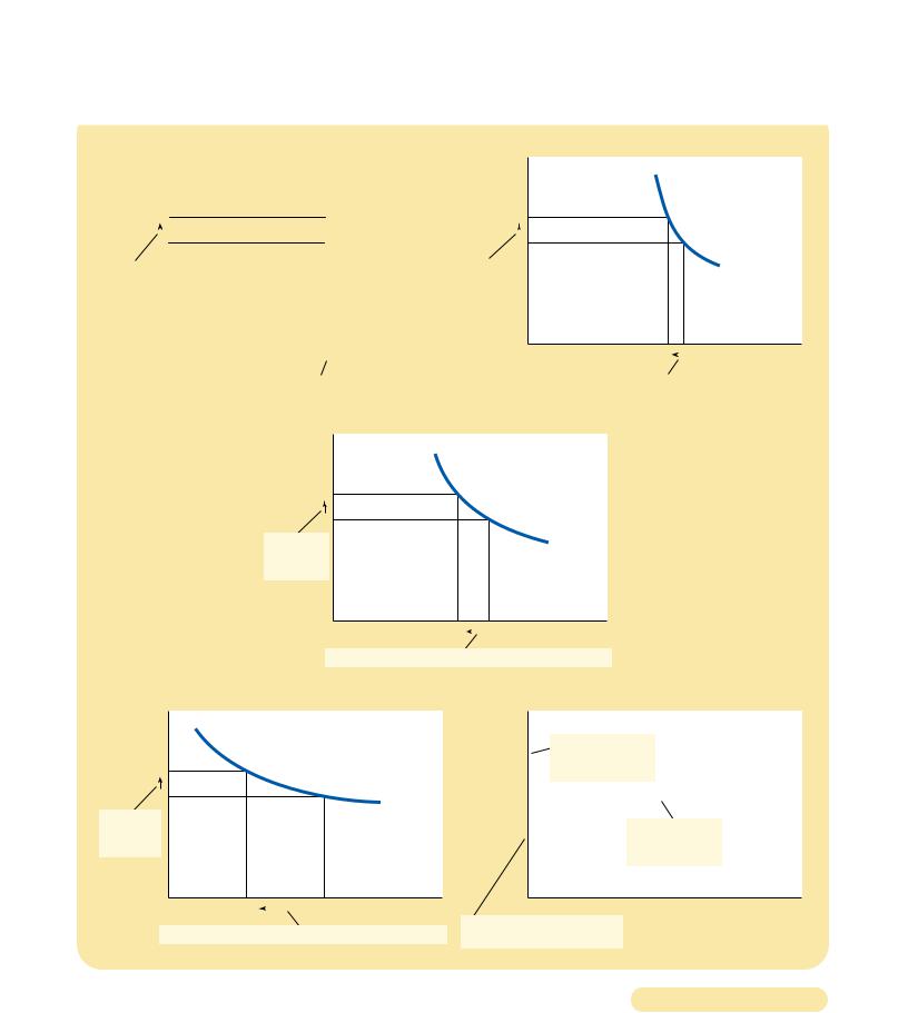
	THE PRICE ELASTICITY OF DEMAND. The price elasticity of demand determines whether		Figur e 5-1
	the demand curve is steep or flat. Note that all percentage changes are calculated using
	the midpoint method.

TLFeBOOK

94	Elasticity and Its Application
98	PART TWO SUPPLY AND DEMAND I: HOW MARKETS WORK

total r evenue

the amount paid by buyers and received by sellers of a good, computed as the price of the good times the quantity sold

The numerator is the percentage change in quantity computed using the midpoint method, and the denominator is the percentage change in price computed using the midpoint method. If you ever need to calculate elasticities, you should use this formula.

Throughout this book, however, we only rarely need to perform such calculations. For our purposes, what elasticity represents—the responsiveness of quantity demanded to price—is more important than how it is calculated.

THE VARIETY OF DEMAND CURVES

Economists classify demand curves according to their elasticity. Demand is elastic when the elasticity is greater than 1, so that quantity moves proportionately more than the price. Demand is inelastic when the elasticity is less than 1, so that quantity moves proportionately less than the price. If the elasticity is exactly 1, so that quantity moves the same amount proportionately as price, demand is said to have unit elasticity.

Because the price elasticity of demand measures how much quantity demanded responds to changes in the price, it is closely related to the slope of the demand curve. The following rule of thumb is a useful guide: The flatter is the demand curve that passes through a given point, the greater is the price elasticity of demand. The steeper is the demand curve that passes through a given point, the smaller is the price elasticity of demand.

Figure 5-1 shows five cases. In the extreme case of a zero elasticity, demand is perfectly inelastic, and the demand curve is vertical. In this case, regardless of the price, the quantity demanded stays the same. As the elasticity rises, the demand curve gets flatter and flatter. At the opposite extreme, demand is perfectly elastic. This occurs as the price elasticity of demand approaches infinity and the demand curve becomes horizontal, reflecting the fact that very small changes in the price lead to huge changes in the quantity demanded.

Finally, if you have trouble keeping straight the terms elastic and inelastic, here’s a memory trick for you: Inelastic curves, such as in panel (a) of Figure 5-1, look like the letter I. Elastic curves, as in panel (e), look like the letter E. This is not a deep insight, but it might help on your next exam.

TOTAL REVENUE AND THE PRICE ELASTICITY OF DEMAND

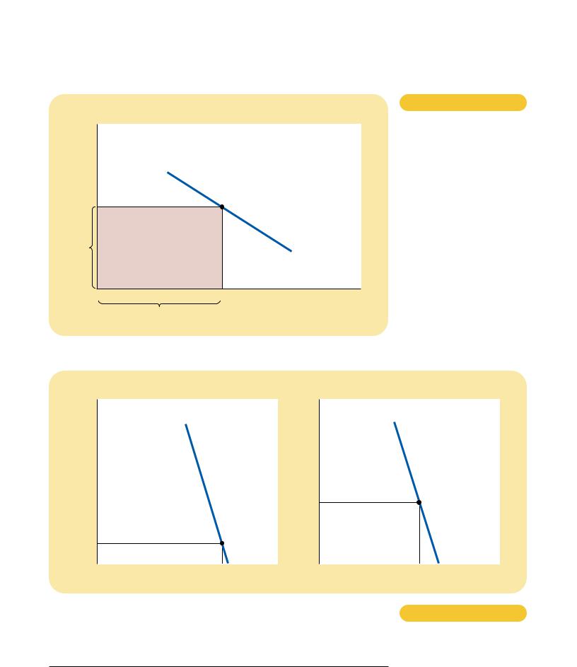
When studying changes in supply or demand in a market, one variable we often want to study is total revenue, the amount paid by buyers and received by sellers of the good. In any market, total revenue is P Q, the price of the good times the quantity of the good sold. We can show total revenue graphically, as in Figure 5-2. The height of the box under the demand curve is P, and the width is Q. The area of this box, P Q, equals the total revenue in this market. In Figure 5-2, where P $4 and Q 100, total revenue is $4 100, or $400.

How does total revenue change as one moves along the demand curve? The answer depends on the price elasticity of demand. If demand is inelastic, as in Figure 5-3, then an increase in the price causes an increase in total revenue. Here an increase in price from $1 to $3 causes the quantity demanded to fall only from 100

TLFeBOOK

Elasticity and Its Application	95
CHAPTER 5 ELASTICITY AND ITS APPLICATION	99

Figur e 5-2

Price

$4

P

0

Price

$1

0

TOTAL REVENUE. The total amount paid by buyers, and received as revenue by sellers, equals the area of the box under the demand curve, P Q. Here, at a price of $4, the quantity demanded is 100, and total revenue is $400.

P Q $400
(revenue)	Demand

100

Quantity

Q

Price

					$3
							Revenue $240
		Demand							Demand
Revenue $100
	100		Quantity		0		80		Quantity

HOW TOTAL REVENUE CHANGES WHEN PRICE CHANGES: INELASTIC DEMAND. With an

inelastic demand curve, an increase in the price leads to a decrease in quantity demanded that is proportionately smaller. Therefore, total revenue (the product of price and quantity) increases. Here, an increase in the price from $1 to $3 causes the quantity demanded to fall from 100 to 80, and total revenue rises from $100 to $240.

Figur e 5-3

TLFeBOOK

96	Elasticity and Its Application
100	PART TWO SUPPLY AND DEMAND I: HOW MARKETS WORK

to 80, and so total revenue rises from $100 to $240. An increase in price raises P Q because the fall in Q is proportionately smaller than the rise in P.

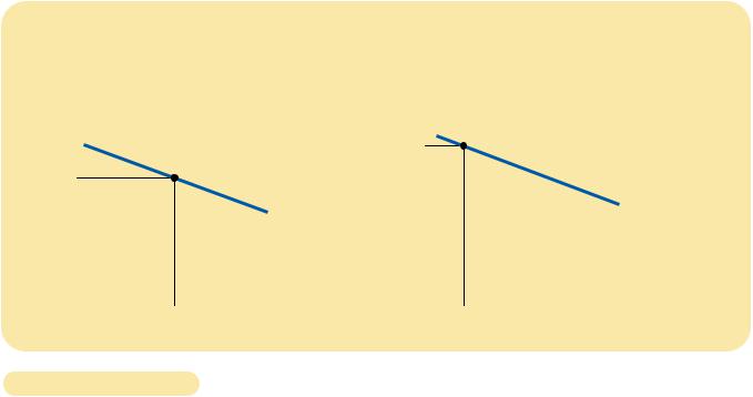
We obtain the opposite result if demand is elastic: An increase in the price causes a decrease in total revenue. In Figure 5-4, for instance, when the price rises from $4 to $5, the quantity demanded falls from 50 to 20, and so total revenue falls from $200 to $100. Because demand is elastic, the reduction in the quantity demanded is so great that it more than offsets the increase in the price. That is, an increase in price reduces P Q because the fall in Q is proportionately greater than the rise in P.

Although the examples in these two figures are extreme, they illustrate a general rule:

When a demand curve is inelastic (a price elasticity less than 1), a price increase raises total revenue, and a price decrease reduces total revenue.

When a demand curve is elastic (a price elasticity greater than 1), a price increase reduces total revenue, and a price decrease raises total revenue.

In the special case of unit elastic demand (a price elasticity exactly equal to 1), a change in the price does not affect total revenue.

Price					Price
$4			Demand		$5				Demand
	Revenue $200								Revenue $100
0	50		Quantity		0	20			Quantity

Figur e 5-4		HOW TOTAL REVENUE CHANGES WHEN PRICE CHANGES: ELASTIC DEMAND. With an
		elastic demand curve, an increase in the price leads to a decrease in quantity demanded
		that is proportionately larger. Therefore, total revenue (the product of price and quantity)
		decreases. Here, an increase in the price from $4 to $5 causes the quantity demanded to
		fall from 50 to 20, so total revenue falls from $200 to $100.

TLFeBOOK

Elasticity and Its Application	97
CHAPTER 5 ELASTICITY AND ITS APPLICATION	101

Price
$7			Elasticity is
			larger
6			than 1.
5
4					Elasticity is
					smaller
3					than 1.
2
1
0	2	4	6	8	10	12	14
						Quantity

Figur e 5-5

A LINEAR DEMAND CURVE.

The slope of a linear demand curve is constant, but its elasticity is not.

			TOTAL
			REVENUE	PERCENT	PERCENT
			(PRICE	CHANGE IN	CHANGE IN
	PRICE	QUANTITY	QUANTITY)	PRICE	QUANTITY	ELASTICITY	DESCRIPTION
	$7	0	$ 0	15	200	13.0	Elastic
	6	2	12
				18	67	3.7	Elastic
	5	4	20
				22	40	1.8	Elastic
	4	6	24
				29	29	1.0	Unit elastic
	3	8	24
				40	22	0.6	Inelastic
	2	10	20
				67	18	0.3	Inelastic
	1	12	12
				200	15	0.1	Inelastic
	0	14	0

COMPUTING THE ELASTICITY OF A LINEAR DEMAND CURVE

Table 5-1

NOTE: Elasticity is calculated here using the midpoint method.

ELASTICITY AND TOTAL REVENUE ALONG

A LINEAR DEMAND CURVE

Although some demand curves have an elasticity that is the same along the entire curve, that is not always the case. An example of a demand curve along which elasticity changes is a straight line, as shown in Figure 5-5. A linear demand curve has a constant slope. Recall that slope is defined as “rise over run,” which here is the ratio of the change in price (“rise”) to the change in quantity (“run”). This particular demand curve’s slope is constant because each $1 increase in price causes the same 2-unit decrease in the quantity demanded.

TLFeBOOK

98	Elasticity and Its Application
102	PART TWO SUPPLY AND DEMAND I: HOW MARKETS WORK

Even though the slope of a linear demand curve is constant, the elasticity is not. The reason is that the slope is the ratio of changes in the two variables, whereas the elasticity is the ratio of percentage changes in the two variables. You can see this most easily by looking at Table 5-1. This table shows the demand schedule for the linear demand curve in Figure 5-5 and calculates the price elasticity of demand using the midpoint method discussed earlier. At points with a low price and high quantity, the demand curve is inelastic. At points with a high price and low quantity, the demand curve is elastic.

Table 5-1 also presents total revenue at each point on the demand curve. These numbers illustrate the relationship between total revenue and elasticity. When the price is $1, for instance, demand is inelastic, and a price increase to $2 raises total revenue. When the price is $5, demand is elastic, and a price increase to $6 reduces total revenue. Between $3 and $4, demand is exactly unit elastic, and total revenue is the same at these two prices.

IF THE PRICE OF ADMISSION WERE HIGHER,

HOW MUCH SHORTER WOULD THIS LINE BECOME?

income elasticity of demand

a measure of how much the quantity demanded of a good responds to a change in consumers’ income, computed as the percentage change in quantity demanded divided by the percentage change in income

CASE STUDY PRICING ADMISSION TO A MUSEUM

You are curator of a major art museum. Your director of finance tells you that the museum is running short of funds and suggests that you consider changing the price of admission to increase total revenue. What do you do? Do you raise the price of admission, or do you lower it?

The answer depends on the elasticity of demand. If the demand for visits to the museum is inelastic, then an increase in the price of admission would increase total revenue. But if the demand is elastic, then an increase in price would cause the number of visitors to fall by so much that total revenue would decrease. In this case, you should cut the price. The number of visitors would rise by so much that total revenue would increase.

To estimate the price elasticity of demand, you would need to turn to your statisticians. They might use historical data to study how museum attendance varied from year to year as the admission price changed. Or they might use data on attendance at the various museums around the country to see how the admission price affects attendance. In studying either of these sets of data, the statisticians would need to take account of other factors that affect attendance— weather, population, size of collection, and so forth—to isolate the effect of price. In the end, such data analysis would provide an estimate of the price elasticity of demand, which you could use in deciding how to respond to your financial problem.

OTHER DEMAND ELASTICITIES

In addition to the price elasticity of demand, economists also use other elasticities to describe the behavior of buyers in a market.

The Income Elasticity of Demand Economists use the income elasticity of demand to measure how the quantity demanded changes as consumer income changes. The income elasticity is the percentage change in quantity demanded divided by the percentage change in income. That is,

TLFeBOOK

Elasticity and Its Application	99
CHAPTER 5 ELASTICITY AND ITS APPLICATION	103

IN THE NEWS

On the Road with Elasticity

HOW SHOULD A FIRM THAT OPERATES A

private toll road set a price for its service? As the following article makes clear, answering this question requires an understanding of the demand curve and its elasticity.

F o r W h o m t h e B o o t h To l l s , P r i c e R e a l l y D o e s M a t t e r

BY STEVEN PEARLSTEIN

All businesses face a similar question: What price for their product will generate the maximum profit?

The answer is not always obvious: Raising the price of something often has the effect of reducing sales as pricesensitive consumers seek alternatives or simply do without. For every product, the extent of that sensitivity is different. The trick is to find the point for each where the ideal tradeoff between profit margin and sales volume is achieved.

Right now, the developers of a new private toll road between Leesburg and

Washington-Dulles International Airport are trying to discern the magic point. The group originally projected that it could charge nearly $2 for the 14-mile one-way trip, while attracting 34,000 trips on an average day from overcrowded public roads such as nearby Route 7. But after spending $350 million to build their much heralded “Greenway,” they discovered to their dismay that only about a third that number of commuters were willing to pay that much to shave 20 minutes off their daily commute. . . .

It was only when the company, in desperation, lowered the toll to $1 that it came even close to attracting the expected traffic flows.

Although the Greenway still is losing money, it is clearly better off at this new point on the demand curve than it was when it first opened. Average daily revenue today is $22,000, compared with $14,875 when the “special introductory” price was $1.75. And with traffic still light even at rush hour, it is possible that the owners may lower tolls even further in search of higher revenue.

After all, when the price was lowered by 45 percent last spring, it generated a 200 percent increase in volume three months later. If the same ratio applies again, lowering the toll another 25 percent would drive the daily volume up to 38,000 trips, and daily revenue up to nearly $29,000.

The problem, of course, is that the same ratio usually does not apply at

every price point, which is why this pricing business is so tricky. . . .

Clifford Winston of the Brookings Institution and John Calfee of the American Enterprise Institute have considered the toll road’s dilemma. . . .

Last year, the economists conducted an elaborate market test with 1,170 people across the country who were each presented with a series of options in which they were, in effect, asked to make a personal tradeoff between less commuting time and higher tolls.

In the end, they concluded that the people who placed the highest value on reducing their commuting time already had done so by finding public transportation, living closer to their work, or selecting jobs that allowed them to commute at off-peak hours.

Conversely, those who commuted significant distances had a higher tolerance for traffic congestion and were willing to pay only 20 percent of their hourly pay to save an hour of their time.

Overall, the Winston/Calfee findings help explain why the Greenway’s original toll and volume projections were too high: By their reckoning, only commuters who earned at least $30 an hour (about $60,000 a year) would be willing to pay $2 to save 20 minutes.

SOURCE: The Washington Post, October 24, 1996, p. E1.

	Income elasticity of demand	Percentage change in quantity demanded	.
		Percentage change in income

As we discussed in Chapter 4, most goods are normal goods: Higher income raises quantity demanded. Because quantity demanded and income move in the same direction, normal goods have positive income elasticities. A few goods, such as bus

TLFeBOOK