UNIPROCESSOR SCHEDULING

63

task
T1			T
			1
T2	T	2,1			T	2,2	T	2,1			T
											2,2
T3				T					T	3,2
				3,1
	0	1	2	3	4	5	6	7	8	9	time
											10 11 12

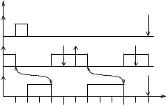
Figure 3.18 Infeasible EDF schedule for tasks with rendezvous constraints.

Here the longest period is 12, which is also the LCM of all three periods. Thus, we generate the following scheduling blocks:

T1(1)

T2(1), T2(2), T2(3), T2(4)

T3(1), T3(2).

Now we specify the rendezvous constraints between blocks:

T2(1) → T3(2),

T3(1) → T2(2),

T2(3) → T3(3), and

T3(2) → T2(4).

Without revising the deadlines, the EDF algorithm yields an infeasible schedule, as shown in Figure 3.18. Using the revised deadlines, the ED algorithm produces the schedule shown in Figure 3.19.

3.2.5 Periodic Tasks with Critical Sections: Kernelized Monitor Model

We now consider the problem of scheduling periodic tasks that contain critical sections. In general, the problem of scheduling a set of periodic tasks employing only semaphores to enforce critical sections is nondeterministic polynomial-time decidable (NP)-hard [Mok, 1984]. Here we present a solution for the case in which the length of a task’s critical section is fixed [Mok, 1984]. A system satisfying this constraint is the kernelized monitor model, in which an ordinary task requests service from a monitor by attempting to rendezvous with the monitor. If two or more tasks request service from the monitor, the scheduler randomly selects one task to ren-

64 REAL-TIME SCHEDULING AND SCHEDULABILITY ANALYSIS

task
T1											T
											1
T2	T	2,1			T				T	2,1	T
					2,2						2,2
T3			T					T
			3,1					3,2
	0	1	2	3	4	5	6	7	8	9	time
											10 11 12

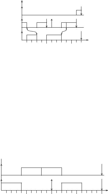
Figure 3.19 EDF schedule for tasks with rendezvous constraints, after revising deadlines.

dezvous with the monitor. Even though a monitor does not have an explicit timing constraint, it must meet the current deadline of the task for which it is performing a service.

Example. Consider the following two periodic tasks:

T1: c1,1 = 4, c1,2 = 4, d1 = 20, p1 = 20,

T2: c2 = 4, d2 = 4, p2 = 10.

The second scheduling block of T1 and the scheduling block of T2 are critical sections.

If we use the EDF algorithm without considering the critical sections, the schedule produced will not meet all deadlines, as shown in Figure 3.20.

At time 8 after completing the second block of T1, the second instance of T2 has not arrived yet so the EDF algorithm executes the next ready task with the earliest deadline, which is the second block of T1. When the second instance of T2 arrives, T1 is still executing its critical section (the second block), which cannot be preempted. At time 12, T2 is scheduled and it misses its deadline at time 15.

task
T1		T1,1	T1,2
T2	T2			T2
	0	5	10	15	time
					20

Figure 3.20 Infeasible EDF schedule for tasks with critical sections.

UNIPROCESSOR SCHEDULING

65

Algorithm:

1.Sort the scheduling blocks in [0, L] in (forward) topological order, so the block with the earliest request times appears first.

2.Initialize the request times of the kth instance of each block Ti, j in [0, L] to (k − 1)pi .

3.Let S and S be scheduling blocks in [0, L]; the computation time and deadline of S

are respectively denoted by cS and dS . Considering the scheduling blocks in (forward)

topological order, revise the corresponding request times by rS = max(rS , {rS + q :

S → S}).

4.Sort the scheduling blocks in [0, L] in reverse topological order, so the block with the latest deadline appears first.

5.Initialize the deadline of the kth instance of each scheduling block of Ti to (k−1)pi +di .

6.Let S and S be scheduling blocks; the computation time and deadline of S are respec-

tively denoted by cS and dS . Considering the scheduling blocks in reverse topological order, revise the corresponding deadlines by dS = min(dS , {dS − q : S → S }).

7.Use the EDF scheduler to schedule the blocks according to the revised request times and deadlines. Do not schedule any block if the current time instant is within a forbidden region.

Figure 3.21 Scheduling algorithm for tasks with critical sections.

task
T1	T1,1			T1,2
T2	T2		T2
0	5	10	15	time
				20

Figure 3.22 Schedule for tasks with critical sections.

Therefore, we must revise the request times as well as the deadlines, and designate certain time intervals as forbidden regions reserved for critical sections of tasks. For each request time rs , the interval (ks , rs ), 0 ≤ rs −ks < q, is a forbidden region if the scheduling of block S cannot be delayed beyond ks + q. The scheduling algorithm is shown in Figure 3.21.

Example. This algorithm produces a feasible schedule, shown in Figure 3.22, for the above two-task system.

66 REAL-TIME SCHEDULING AND SCHEDULABILITY ANALYSIS

3.3 MULTIPROCESSOR SCHEDULING

Generalizing the scheduling problem from a uniprocessor to a multiprocessor system greatly increases the problem complexity since we now have to tackle the problem of assigning tasks to specific processors. In fact, for two or more processors, no scheduling algorithm can be optimal without a priori knowledge of the (1) deadlines,

(2) computation times, and (3) start times of the tasks.

3.3.1 Schedule Representations

Besides representations of task schedules such as timing diagrams or Gantt charts, an elegant, dynamic representation of tasks exists in a multiprocessor system called the scheduling game board [Dertouzos and Mok, 1989]. This dynamic representation graphically shows the statuses (remaining computation time and laxity) of each task at a given instant.

Example. Consider a two-processor system (n = 2) and three single-instance tasks with the following arrival times, computation times, and absolute deadlines:

J1: S1 = 0, c1 = 1, D1 = 2,

J2: S2 = 0, c2 = 2, D2 = 3, and

J3: S3 = 2, c3 = 4, D3 = 4.

Figure 3.23 shows the Gantt chart of a feasible schedule for this task set. Figure 3.24 shows the timing diagram of the same schedule for this task set. Figure 3.25 shows the scheduling game board representation of this task set at time i = 0. The x-axis shows the laxity of a task and the y-axis shows its remaining computation time.

3.3.2 Scheduling Single-Instance Tasks

Given n identical processors and m tasks at time i, m > n, our objective is to ensure that all tasks complete their execution by their respective deadlines. If m ≤ n (the number of tasks does not exceed the number of processors), the problem is trivial since each task has its own processor.

Processor
1	1	2
2		3
0	1	2	3	4	5	time
Figure 3.23				Gantt chart.

MULTIPROCESSOR SCHEDULING

67

		Task
	1
	2
	3
	0			1		2		3		4		5		time
		Figure 3.24						Timing diagram.
C (Computation)
5										Task		C		D		L
	3									1		1		2		1
4										2		2		3		1
3										3		4		4		0

2 2

1 1

L (Laxity)

0 1 2 3 4 5

Number of processors n =2

Time i = 0

Figure 3.25 Scheduling game board.

Let C(i) denote the remaining computation time of a task at time i, and let L(i) denote the laxity (slack) of a task at time i. On the L-C plane of the scheduling game board, executing any n of the m tasks in parallel corresponds to moving at most n of the m tokens one division (time unit) downward and parallel to the C-axis. Thus, for tasks executed:

L(i + 1) = L(i),

C(i + 1) = C(i) − 1.

The tokens corresponding to the remaining tasks that are not executed move to the left toward the C-axis. Thus, for tasks not executed:

L(i + 1) = L(i) − 1,

C(i + 1) = C(i).

Rules for the Scheduling Game Board Each configuration of tokens on the

L-C plane represents the scheduling problem at a point in time. The rules for the scheduling game (corresponding to the scheduling problem) are:

68REAL-TIME SCHEDULING AND SCHEDULABILITY ANALYSIS

1.Initially, the starting L-C plane configuration with tokens representing the tasks to be scheduled is given.

2.At each step of the game, the scheduler can move n tokens one division downward toward the horizontal axis.

3.The rest of the tokens move leftward toward the vertical axis.

4.Any token reaching the horizontal axis can be ignored, that is, it has completed execution and its deadline has been satisfied.

5.The scheduler fails if any token crosses the vertical axis into the second quadrant before reaching the horizontal axis.

6.The scheduler wins if no failure occurs.

Example. We continue the example above by showing a feasible schedule for the task set in the scheduling game board. Suppose we try to use EDF to schedule this task set. At time 0, since J1 and J2 have earlier absolute deadlines, they are assigned the two available processors and they start to run. Their corresponding tokens move downward according to the scheduling game board rule (2). At this time, J3 is not scheduled so its corresponding token starts to move to the left according to the scheduling game board rule (3). At time 1, as shown in Figure 3.26, J1 finishes execution and J2 has one more time unit to run, but J3 is now to the left of the C-axis with a negative laxity, meaning that it will miss its deadline in the future.

We now show a feasible schedule for this task set in Figure 3.27. Instead of using EDF, we try LL. At time 0, since J3 has the smallest laxity, it is assigned an available processor and starts to run. Since J1 and J2 have the same laxity, one (J1) is chosen randomly to execute in the remaining available processor. Their corresponding tokens move downward according to the scheduling game board rule (2). At this time, J2 is not scheduled so its corresponding token starts to move to the left according to the scheduling game board rule (3).

At time 1, J1 finishes execution. J2 and J3 are the only ready tasks so they are scheduled to run. Their corresponding tokens move downward according to the scheduling game board rule (2). J2 finishes execution at time i = 3 and J3 finishes execution at time i = 4.

			C
3										ED schedule
			4							Time i = 1
			3
			2					2
			1
								1						L
-1			0			1		2	3		4

Figure 3.26 Game board showing deadline miss.

							MULTIPROCESSOR SCHEDULING		69
C
						LL schedule
4				3		Time	i = 1
3
				2
2
1					1			L
0				1	2	3	4
C
						LL schedule
4						Time	i = 2
3
2				3
1				2

L

0

1

2

3

4

Figure 3.27 Game board showing a feasible schedule.

Sufficient Conditions for Conflict-Free Task Sets For two or more processors, no deadline scheduling algorithm can be optimal without a priori knowledge of the deadlines, computation times, and start times of the tasks. If no such a priori knowledge is available, optimal scheduling is possible only if the set of tasks does not have subsets that conflict with each another [Dertouzos and Mok, 1989]. A special case is that in which all tasks have unit computation times. Then the EDF algorithm is optimal even in the multiprocessor case.

To derive a sufficient condition for multiprocessor scheduling of single-instance tasks, we first introduce the following notations, which divide the scheduling game board into 3 regions:

R1(k) = {J j : D j ≤ k},

R2(k) = {J j : L j ≤ k D j > k},

R3(k) = {J j : L j > k}.

Then we define the following function [Dertouzos and Mok, 1989].

Surplus Computing Power Function: Define for every positive integer k,

F (k, i ) = kn − C j − (k − L j ).

R1 R2

This function provides a measure of the surplus computing power of the multiprocessor system in terms of available processor time units between a given time instant i