CHENG–CHEN TIMING ANALYSIS METHODOLOGY			405
layer 1	layer2	layer3	layer4	layer5	layer 5	layer7
r1	r2	r3		r6	r8
			r5			r10
		r4		r7	r9

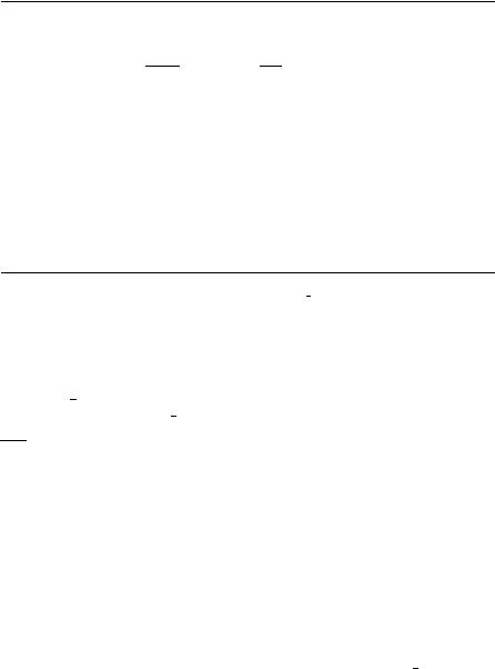
Figure 11.7 PI graph of Waltz program segment.

3. The PI graph of the Waltz program segment is:

	r1 r2 r3 r4 r5 r6 r7 r8 r9 r10
r1	-	m	p p - p p p p p
r2	-	-	p p p			-	- - -			-
r3	-	-	- - m p p p p p
r4	-	-	- - m p p p p p
r5	-	-	- - -			p	p - -			-
r6	-	-	- - -			-	- p p p
r7	-	-	- - -			-	- p p			p
r8	-	-	-	-	-	-	-	-	-	p
r9	-	-	-	-	-	-	-	-	-	p
r10 -		-	-	-	-	-	-	-	-	-

“p” stands for the existence of a p-type edge, “m” the existence of an m-type edge, and “-” no edge at all. For example, r1, r2 is an m-type edge and r5, r6 is a p-type edge.

4.We then transform the PI graph into an n-partite PI graph (shown in Figure 11.7).

Our analysis tool constructs the PI graph of the program automatically.

Our framework for static timing analysis of OPS5 programs is as follows. We first extract the semantic relationships among rules in a program by representing it as a potential instantiation graph. Then, based on the type of the constructed PI graph, we determine whether the program satisfies a termination condition. If it does, we proceed to check its worst-case execution time in terms of the number of rule firings and match comparisons. For programs with potential cycles, we show how the programmer can provide assistance in computing a conservative response time upper bound.

11.3.3 Response Time of OPS5 Systems

In this section, we study the response-time analysis problem in the context of OPS5 production systems. The response time of an OPS5 program is investigated in two

406 TIMING ANALYSIS OF PREDICATE-LOGIC RULE-BASED SYSTEMS

respects: the maximal number of rule firings and the maximal number of basic comparisons made by the Rete network during the execution of this program. Several sets of conditions that guarantee the property of program termination will be given. Each of these sets of conditions thus represents a class of programs. We tackle the response-time analysis problem by first determining whether the given system is in one of the classes with the property of execution termination and then computing an upper bound on the maximal response time, if possible.

The first class shown to have bounded response time is the class of programs with acyclic potential instantiation graphs. An algorithm used to compute response time upper bounds of programs in this class is introduced.

Theorem 2. Let p denote a set of rules. The execution of p always terminates in a bounded number of recognize–act cycles if the potential instantiation graph G Pp I is acyclic.

Proof . The proof is simliar to the proof of termination in [Aiken, Widom, and Hellerstein, 1992]. Basically, the potential instantiation graph has similar behavior as the triggering graph in [Aiken, Widom, and Hellerstein, 1992].

Corollary 1. Let p denote a set of rules. If the execution of p will not terminate in a bounded number of recognize–act cycles, a cycle C exists in the potential instantiation graph G Pp I . Let C = r1, . . . , rk , rk+1 and r1 = rk+1. ri potentially instantiates ri+1, where i = 1 . . . k, and ri will fire infinitely often.

We now present a response-time upper bound algorithm that computes the maximal number of instantiations that may exist during the execution and returns this number as the maximal number of rule firings. A direct result of this strategy is that the upper bound obtained is not affected by the resolution strategy used in the select phase of the recognize–act cycle. No matter what resolution strategy is used, no more than the maximal number of instantiations may exist during the execution. Hence, the maximal number of instantiations that may exist is an upper bound on the number of recognize–act cycles during the execution.

Number of Rule Firings One of the major characteristics of production systems is that the execution time depends on the content of the initial working memory. Not only do the classes (or types) of initial WMEs affect the execution time, but also the number of WMEs of each class plays a role in required execution time. For example, an initial working memory with three WMEs of a certain class and an initial working memory with 30 WMEs of the same class may require different amounts of time for the production system to complete execution. Furthermore, different executions may apply to different sets of initial working memory.

Although the numbers and classes of initial WMEs can only be known at runtime, it is reasonable to assume that the experienced software developer (or user) has an idea of the maximal possible number of initial WMEs of each class in which the application domain may result. In addition, the proposed response-time upper bound algorithm is based on counting the maximal number of instantiations, which

CHENG–CHEN TIMING ANALYSIS METHODOLOGY

407

is increasing with respect to the number of WMEs of each class. The response time upper bound obtained by applying the proposed algorithm to an initial working memory consisting of the maximal possible number of WMEs of each class is a response time upper bound of the system, since all of the executions cannot have a larger number of WMEs than the (already known) maximal possible number of WMEs. Hence, to obtain a response time upper bound of an OPS5 production system, the developers (or users) need to apply the proposed algorithm to an initial working memory consisting of the maximal possible number of WMEs of each class.

Let r denote a rule of p with acyclic PI graph and cri denote the ith nonnegated condition element in the LHS of r. To simplify the explanations later, a working memory element is classified as an old WME if it exists at the invocation; otherwise, it is a new WME since it is produced as a result of rule firings. The WMEs matching cri are called matching WMEs of cri . A WME is a matching WME of r if it is a matching WME of one of the condition elements in the LHS of r.

r can be fired only if it is instantiated, and each instantiation of r can be fired at most once. According to theorem 2, the execution of p always terminates in a bounded number of recognize–act cycles. r can thus be fired at most only a bounded number of times. Hence, only a bounded number of instantiations of r must exist during the execution of p. This means that there are only a bounded number of matching WMEs matching to r during the execution of p. There are only two kinds of matching WMEs of r: old matching WMEs of r, which exist at the invocation, and new matching WMEs of r, which result from the firings of rules during the execution. The number of matching WMEs of r is equal to the number of old matching WMEs of r plus the number of new matching WMEs of r. Hence, the number of old matching WMEs of r plus an upper bound on the number of new matching WMEs of r is an upper bound on the number of matching WMEs of r.

Since G Pp I is acyclic, new matching WMEs of r result from the firings of its predecessors in G Pp I . To find the number of new matching WMEs, G Pp I is drawn as an n-partite graph from left to right. Assume there are n layers in G Pp I . The layers in G Pp I are labeled from left to right as layer 1, layer 2, . . . , layer n. For each i, 1 ≤ i ≤ n, let pi denote the set of rules in layer i, where n is the number of layers in G Pp I (as shown in Figure 11.7). Suppose r is in layer i. If i = 1, no new matching WMEs of r can be produced as a result of rule firings. If i > 1, only the firings of those rules in layer 1 through layer i − 1 can possibly produce new matching WMEs of r. If the numbers of new WMEs to r, respectively resulting from the firings of rules in layer 1 through layer i − 1, have all been calculated, the number of matching WMEs of r can be easily calculated. Once we obtain the number of matching WMEs of r, we can calculate an upper bound on the number of firings by r. Furthermore, if i < n, we can compute upper bounds on the numbers of new WMEs, resulting from the firing(s) of r, to rules in layer i + 1 through layer n. Hence, the numbers of matching WMEs of individual rules and the upper bounds on the numbers of rule firings are computed in the order corresponding to positions of the rules in G Pp I . From left to right, the numbers of matching WMEs (and the upper bounds on the numbers of firings) to rules in layer 1 are computed first, then to rules in layer 2, and so on.

408 TIMING ANALYSIS OF PREDICATE-LOGIC RULE-BASED SYSTEMS

An Upper Bound on the Number of Firings by r Assume there are k nonnegated condition elements (ignore the negated condition elements) in the LHS of r. For each i, 1 ≤ i ≤ k, let Nri denote the number of matching WMEs of cri , and dri denote the number of matching WMEs of cri that are removed from the working memory as a result of one firing of r. There are at most Nr1 Nr2 · · · Nrk instantiations of r with respect to this working memory. However, if dri is not equal to 0, there can be at most Nri /dri firings of r before all of the matching WMEs of cri are deleted as a result of these firings. This means that there can be at most

Ir = min(Nr1 Nr2 · · · Nrk , Nr1/dr1 , Nr2/dr2 , . . . , Nrk /drk )

(11.1)

firings of r, unless the firings of rules result in new WMEs that result in new instantiation(s) of r. Note that Nri /dri ≡ ∞ if dri is equal to 0.

Example 16. Assume there are three WMEs of the class E1, four WMEs of the class E2, and three WMEs of the class E3 in the current working memory. Consider the following two rules in the production memory.

(P r1	(E1 · · ·) (E2	· · ·) (E2	· · ·) –(E3 · · ·) −→ (make · · ·) (make · · ·) )
(P r2	(E1 · · ·) (E2	· · ·) (E3	· · ·) −→ (make E4 · · ·) (remove 2) )

Without knowing the contents of these WMEs, there are at most Nr11 Nr21 Nr31 = 3 4 4 = 48 instantiations of r1 with respect to this working memory. Since each firing of r1 does not delete any WME, at most 48 firings of r1 exist. Similarly, at most Nr12 Nr22 Nr32 = 3 4 3 = 36 instantiations of r2 exist with respect to this working memory. However, each firing of r2 removes a WME of the class E2. Hence, there are at most min(36, 4/1 ) = 4 firings of r2 with respect to this working memory.

Maximal Numbers of New Matching WMEs Assume it has been determined (by the above method) that there are at most Ir possible instantiations/firings of r during the execution of p. An RHS action with the command make results in a new WME and increases the number of WMEs of the specified class by one, an RHS action with the command modify modifies the content of a WME and does not changes the number of WMEs of the specified class, and an RHS action with the command remove removes a WME and decreases the number of WMEs of the specified class by one. Since there are at most Ir possible instantiations of r, r can be fired a total of 0 to Ir times. It is possible that none of the Ir possible instantiations exists. If this is the case, r will not be fired. This means that the number of WMEs of each class will not be affected by r in the worst case in terms of the capability of reducing the number of WMEs even though the RHS of r contains an action(s) with the command remove. On the other hand, if the RHS of r contains x actions with the command make on the class E, then each firing of r results in x new WMEs of the class E. This means that a maximum of x Ir new WMEs of the class E may be created as a result of the firings of r. Therefore, for the purpose of obtaining the maximal number of WMEs that may affect the instantiatibility of rules,

CHENG–CHEN TIMING ANALYSIS METHODOLOGY

409

only the actions with the command make need to be considered. Let NEr denote the number of actions, in the RHS of r, with the command make that produce WMEs of the class E.

Example 17. Assume there are two WMEs of class E1, 2 WMEs of class E2, and one WMEs of class E3 in the current working memory. Let r3 below be one of the rules in the production memory.

(P r3 (E1 · · ·) (E2 · · ·) (E2 · · ·) −→ (modify 1 · · ·) (remove 2) (make E3 · · ·) )

There are at most min(2 2 2, 2/1 ) = 2 firings of r3 with respect to this working memory. Each firing of r3 produces a new WME of the class E3. There are at most mr33 Ir3 = 1 2 = 2 new WMEs of the class E3 as a result of these firings of r3. Hence, there are at most two WMEs of class E1, two WMEs of class E2, and three WMEs of class E3 after these firings of r3.

For each rule r in layer i, we compute the maximal number of new WMEs that result from the firing(s) of r for each working memory element class. For each class E, the sum of those maximal numbers of new WMEs of E, respectively produced by the firings of rules in layer i, is an upper bound on the number of new WMEs of E produced by layer i. Applying the above method, we can find the maximal number of new WMEs of each class produced as a result of the firings of each rule. However, not all of the new WMEs produced as a result of the firings of one rule, say r1, may be new matching WMEs of all of the other rules. Let r1 denote a rule whose RHS contains an action that matches one of the nonnegated condition elements in the LHS of r2. If r1 is in a layer higher than r2, those WMEs produced as a result of the firings of r1 cannot be used to instantiate r2; otherwise there would be a path from r1 to r2 in G Pp I , meaning that r1 would be in a layer lower than r2. Hence, the firings of rules can produce new matching WMEs only to rules in higher levels.

Assume r1 is in a layer lower than r2. A new matching WME of the nonnegated condition element cri2 in the LHS of r2 may result from an action, say arj1 , that matches cri2 , with the command make or modify in the RHS of r1. If arj1 is a make action, the resulting WME is a new matching WME of cri2 . This means that the number of new matching WMEs of cri2 should be increased by one due to arj1 , as a result of each firing of r1. If the RHS of r1 contains x make actions that match cri2 , the number of new matching WMEs of cri2 should be increased by x Ir1 as a result of the firings of r1.

If arj1 is a modify action on a WME that matches cri2 , the presence of arj1 does not change the number of matching WMEs of cri2 . If arj1 is a modify action on a WME that does not match cri2 , the resulting WME is a new matching WME of cri2 . This means that the number of new matching WMEs of cri2 should also be increased by

one due to arj1 , as a result of each firing of r1. If the RHS of r1 contains x modify actions that (1) match cri2 and (2) modify WMEs that do not match cri2 , the number

410 TIMING ANALYSIS OF PREDICATE-LOGIC RULE-BASED SYSTEMS

Input An OPS5 program, p.

Output An upper bound, B, on the number of firings by p.

1.Set B to 0, and, for each class Ec, let NEc be the number of old WMEs.

2.For each rule r layer 1, initialize Nrk for each k condition element.

3.Determine all of the Nrkj ,ri s and all of the NEri s.

4.Construct the PI graph G Pp I . Let n be the number of layers in G Pp I .

5.For l := 1 to n, Do

For each rule ri layer l, Do

(a)Iri := min(Nr1i Nr2i · · · Nrki , Nr1i /dr1i , Nr2i /dr2i , . . . , Nrki /drki );

(b)B := B + Iri ;

		ri
(c)	For each class Ec, Do NEc := NEc + Iri NEc		;
(d)	For each rule r j layer m, m > l, Do Nrkj := Nrkj +			Nrkj ,ri	Iri , for all k.

6. Output(B).

Figure 11.8 Algorithm A.

of new matching WMEs of cri2 should be increased by x Ir1 as a result of the firings of r1.

Algorithm A Based on the strategy described above, we have developed the following algorithm, Algorithm A (see Figure 11.8), to compute an upper bound on the number of recognize–act cycles during the execution of OPS5 programs. Note that

Nik, j denotes the number of new matching WMEs of the kth condition element of ri produced as a result of one firing of r j .

An Example We now show the analysis of a program segment of Waltz, an expert system that implements the Waltz labeling [Winston, 1977] algorithm. This program analyzes the lines of a two-dimensional drawing, and labels them as if they were edges in a three-dimensional object. The analyzed program segment is a subset of 10 rules of Waltz, which has 33 rules, to demonstrate the proposed algorithm. These rules perform the task of finding the boundaries and junctions of objects. For the sole purpose of demonstrating the proposed analysis algorithm, the understanding of the semantics of the Waltz algorithm (or program) is not necessary.

Assume, at the invocation, the working memory consists of 20 WMEs of the class line and the following WME: (stage duplicate). Following Algorithm A, the potential instantiation graph of this program segment is built and shown in Figure 11.7. Tables 11.1 and 11.2 show some of the characteristics of this program segment. For each condition element crji of each rule ri , the number of removed matching WMEs

				CHENG–CHEN TIMING ANALYSIS METHODOLOGY													411
TABLE 11.1 Program characteristics—1 of Waltz program
segment
	Matching WMEs removed								WMEs increment
	d1	d2	d3	d4	d5
								Nri		Nri		Nri		Nri
	ri	ri	ri	ri	ri			Es		El		Ee		E j
r1	0	1				0			0		2			0
r2	1					0			0		0			0
r3	0	3	3	3		0			0		0			1
r4	0	2	2			0			0		0			1
r5	1					0			0		0			0
r6	1	0	2	2		0			0		0			0
r7	1	0	3	3	3	0			0		0			0
r8	1	0	2	2		0			0		0			0
r9	1	0	3	3	3	0			0		0			0
r10	0	2	2			0			0		0			0

of crji as a result of one firing of ri is shown. Also shown are the respective numbers of new WMEs of each class and respective numbers of new matching WMEs of condition elements of rules respectively produced as a result of each firing of individual rules. For example, Table 11.1 indicates that each firing of r4 removes two matching WMEs from both the second and the third condition elements of r4. It is also shown that each firing of r4 may increase the number of WMEs of the class junction by one.

TABLE 11.2 Program characteristics—2 of Waltz program segment

Number of new matching WMEs produced per rule firing

r1 Nr23,r1 , Nr33,r1 , Nr43,r1 , Nr24,r1 , Nr34,r1 , Nr36,r1 , Nr46,r1 , Nr37,r1 , Nr47,r1 ,

Nr57,r1 , Nr38,r1 , Nr48,r1 , Nr39,r1 , Nr49,r1 , Nr59,r1 , Nr210,r1 , Nr310,r1 : 2

r

2

N 1

,r2

, N 1

,r2

, N 1

,r2

: 1

r3

r4

r5

r

3

N 2

,r3

,

N 2

,r3

: 1

r7

r9

r

4

N 2

,r4

,

N 2

,r4

: 1

r6

r8

r

5

N 1

,r5

,

N 1

,r5

: 1

r6

r7

r

6

N 1

,r6

,

N 1

,r6

: 1

N 2

,r6

: 2

r8

r9

r10

r

7

N 1

,r7

,

N 1

,r7

: 1

N 2

,r7

: 3

r8

r9

r10

r

8

N 1

: 1

N 2

,r8

: 2

r10,r8

r10

r

9

N 1

: 1

N 2

,r9

: 3

r10,r9

r10

r10

412	TIMING ANALYSIS OF PREDICATE-LOGIC RULE-BASED SYSTEMS
TABLE 11.3		Analysis results
																	Number of
		Number of matching WMEs						Number of WMEs after firings									firings
		N 1	N 2	N 3	N 4	N 5		N	Es	N	El	N	Ee	N	E j		I	B
		ri	ri	ri	ri	ri											ri
Invocation							1			20		0		0
Layer 1	r1	1	20				1			20		40		0		20		20
Layer 2	r2	1					1			20		40		0		1		21
Layer 3	r3	1	40	40	40		1			20		40		14		14
	r4	1	40	40			1			20		40		20		20
							1			20		40		34		55
Layer 4	r5	1					1			20		40		34		1		56
Layer 5	r6	1	20	40	40		1			20		40		34		1
	r7	1	14	40	40	40	1			20		40		34		1
							1			20		40		34		58
Layer 6	r8	2	20	40	40		1			20		40		34		2
	r9	2	14	40	40	40	1			20		40		34		2
							1			20		40		34		62
Layer 7	r10	4	55	40			1			20		40		34		20		82

Another table showing the initial values of Nrk s for all rules and k is created. This table will be modified throughout the analysis process. Due to space limitation, it is not shown in this dissertation. Instead, we incorporate the final values of Nrk s in Table 11.3, which shows the analysis results. From this table, Algorithm A determines that there are at most 82 rule firings by this program segment during the execution if there are only 1 WME of the class stage and 20 WMEs of the class line at the invocation.

Match Time In this section, we compute an upper bound on the time required during the match phase in terms of the number of comparisons made by the Rete algorithm [Forgy, 1982]. Each comparison is a basic testing operation, such as testing whether the value of the attribute ↑age is greater than 20, whether the value of ↑sex is M, and so on.

The Rete Network The Rete Match algorithm is an algorithm to compare a set of LHSs to a set of elements to discover all the instantiations. The given OPS5 program is compiled into a Rete network which receives as input the changes to the working memory and produces as output the modifications to the conflict set. The descriptions of the working memory changes are called tokens. A token consists of a tag and a working memory element. The tag of a token is used to indicate the addition or deletion of the working memory element of the token. When an element is modified, two tokens are sent to the network: one token with tag − indicates that the old element has been deleted from working memory and one token with tag + indicates that the new element has been added. The Rete algorithm uses a tree-structured network (refer to Figure 11.9). Each Rete network has a root node and several terminal nodes. The root node distributes to other nodes the tokens that are passed to the net-

	CHENG–CHEN TIMING ANALYSIS METHODOLOGY		413
	Root
1	2	3
Department	Teacher	Student
4		5
1:^dep_id=2:^dep_id		^sex=M

6

2:^class=3:^class

r4

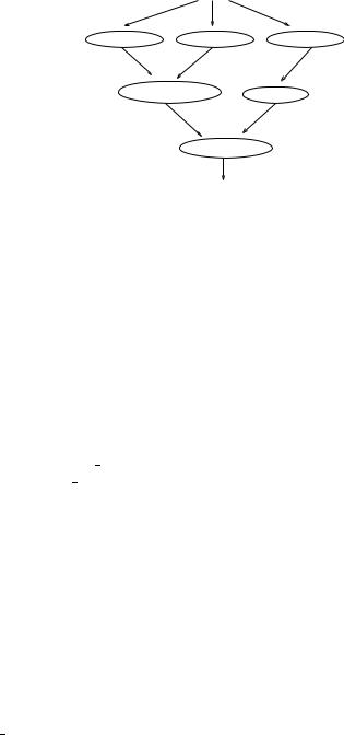
Figure 11.9 The Rete network for r4.

work. Each of the terminal nodes reports the satisfaction of the LHS of some rule. Other than the root node and terminal nodes, two types of nodes are present in the Rete network: one-input nodes and two-input nodes. Each one-input node tests for the presence of one intra-element feature, while each two-input node tests the interelement feature(s) applying to the elements it processes. Each of the intra-element features involves only one working memory element. The inter-element features are the conditions involving more than one working memory element.

Example 18. Consider the following rule.

(P r4

(Department ↑dep id D ) (Teacher ↑dep id D ↑class C )

(Student ↑sex M ↑class C )

−→

· · ·)

Rule r4 is compiled into a Rete network and shown in Figure 11.9. In this figure, the Root node of the network receives the tokens that are sent to this network and passes copies of the tokens to of all its successors. The successors of the Root node are classchecking nodes, which are nodes 1, 2, and 3. Tokens satisfying the class-checking test are passed to the Root node’s successors (test that the class of the element is Department, Teacher, or Student). The successors of class-checking nodes are a oneinput node (node 5) and a two-input node (node 4). The one-input node tests the intraelement feature (tests the attribute of ↑sex) and sends the tokens to its successors. The two-input node compares tokens from different paths and joins them to create bigger tokens if they satisfy the inter-element constraints of the LHS (test the attribute of ↑dep id). Node 6 is a two-input node that joins tokens from node 4 and node 5 if they satisfy the inter-element feature (test the attribute of ↑class). The terminal node (node r4) will receive tokens that instantiate the LHS of r4. The terminal node

414 TIMING ANALYSIS OF PREDICATE-LOGIC RULE-BASED SYSTEMS

sends out the information that the conflict set must be changed. Actually, the Rete algorithm performs the match by processing one token at a time and traversing the entire network depth-first.

The Rete network must maintain state information because it must know what is added to or deleted from working memory. Each two-input node maintains two lists, one called L-list, of tokens coming from its left input, and the other called R-list, of tokens coming from its right input. The two-input nodes use the tag to determine how to modify their internal lists. When a + token is processed, it is stored in the list. When a − token is processed, a token with an identical data part in the list is deleted. More details about the Rete network can be found in [Forgy, 1982].

The Number of Comparisons Since each one-input node tests for the presence of one intra-element feature, one comparison is conducted whenever a token is passed to a one-input node. On the other hand, a two-input node may conduct many comparisons, since many pairs of tokens may have to be checked whenever a token is passed to this node. Each pair of tokens consists of the incoming token and one of the tokens in the maintained list corresponding to the other input. Hence, for each two-input node, we need to know the maximal number of tokens in each of the two maintained lists.

Assume v is a two-input node that checks the presence of vx inter-element features, meaning that v conducts vx comparisons for each pair of tokens. Let Lv and Rv respectively denote the maximal number of tokens in the L-list and R-list maintained by v. Hence, if a token enters the left-input of v, a maximum of Rv pairs of tokens need to be checked. This in turn means that a maximum of Rv vx comparisons needs to be conducted whenever a token enters the left-input of v. If a token enters the right-input of v, a maximum of Lv pairs of tokens needs to be checked, meaning that a maximum of Lv vx comparisons needs to be conducted. Furthermore, the L-list of each of v’s successors has a maximal number of Rv Lv tokens.

If the tokens entering the right-input of v are of the class E, the value of Rv is equal to the maximal number of WMEs of the class E that may exist during the execution. If the left-input of v receives tokens from a one-input node that checks tokens of some class, say E , the value of Lv is equal to the maximal number of WMEs of class E that may exist during the execution. If the left-input of v receives tokens from a two-input node, say v , the value of Lv is equal to the value of Rv Lv .

Example 19. Assume there are at most 50 WMEs of the class Student, 20 WMEs of the class Teacher and 5 WMEs of the class Department in the working memory during the execution. Hence, L4 = 5 and R4 = 20, L6 = 100, R6 = 50 (see Figure 11.9). We compute the maximum number of comparisons by a token of class Department passing to the Rete network as follows. For a token of class Department entering the left-input of node 6, a maximum of 50 tokens of class Student need to be checked, and there is one comparison (to check the attribute of ↑class) in node 6, meaning that a maximum of 50 1 comparisons needs to be conducted. The same applies to node 4. Then it is a maximum of 20 1 comparisons (this one comparison

CHENG–CHEN TIMING ANALYSIS METHODOLOGY

415

check is for the attribute ↑ dep id) performed, and these 20 tokens then enter the left-input of node 6. So, the maximum number of comparisons for a token of class Department passing from node 4 to node 6 is 20 + 20 50 = 1020. There are three class-checking nodes. A maximum of 1023 comparisons will be conducted by a token of class Department passing to this Rete network. Therefore, a maximum of 258 and 104 comparisons will be conducted by the same network if a token of the class Teacher and class Student is passed to this network. Furthermore, a token of any class other than Student, Teacher, and Department results in only three comparisons by the network since the token will be discarded at the three class-checking nodes.

Based on the discussion above, we compute an upper bound on the number of comparisons made in the match phase as follows. Assume p is an n-rule OPS5 program. For each rule r, let Rr represent the Rete sub-network that corresponds to r. For each class α of tokens, we first compute an upper bound on the number of comparisons made by Rr during the match phase. Let Trα denote this upper bound. The sum of Trαs, one for each rule r p, is an upper bound on the number of comparisons made by the Rete network when a token of class α is processed by the network. Let T α denote this upper bound. That is,

T α = Trα. (11.2)

r p

Since there are only a finite number of actions in the RHS of each rule, each firing of a rule produces only a finite number of tokens. Each of these tokens is then passed to and processed by the Rete network. Having obtained all of the T αs, we can compute, for each rule r p, an upper bound on the number of comparisons made by the network as a result of the firing of r by summing up (nrα T α)s where, for each α, nrα denotes the number of tokens of the class α added or deleted as a result of the firing of r. For example, assume there are three classes of WMEs, E1, E2, and E3.

(P r1

(E1 ↑ value duplicate)

(E2 ↑ p1 P1 ↑ p2 P2 )

−→

(make E3 ↑ p1 P ↑ p2 P2 ) (make E3 ↑ p1 P2 ↑ p2 P1 ) (modify 1 ↑ value detect junctions) (remove 2))

Then nrE11 is 2, nrE12 is 1, nrE13 is 2 as a result of firing r1. nrE11 is 2 because when an element of class E1 is modified, two tokens are produced, one token indicating that the old form of the element has been deleted from WM, and the other token indicating that the new form of the element has been added to WM. nrE12 is 1 since an element of class E2 is removed from WM, and one token is produced to indicate deletion. nrE13 is 2 because two elements have been added to WM, and two tokens are

416 TIMING ANALYSIS OF PREDICATE-LOGIC RULE-BASED SYSTEMS

produced to indicate addition. Let Tr denote this upper bound. That is,

Tr = nrα T α. (11.3)

α

In this case, we can obtain Tr1 from expression (11.3) by computing Tr1 = nrE11

T E1 + nrE22 T E2 + nrE33 T E3 . Let Tp denote an upper bound on the number of comparisons made by the Rete network during the execution. Since the maximal

number of firings by each rule can be obtained by applying Algorithm A, we can easily compute the value of Tp. That is,

Tp = Ir Tr . (11.4)

r p

Algorithm M To compute the maximal number of comparisons made by the Rete network Rp in each recognize–act cycle when a token is passed to and processed by Rp, we need to add the numbers of comparisons respectively performed by individual nodes in Rp. Assume a token of class α is passed to Rp. The token passes to the network from top to bottom, but the computing of Trα is from bottom to top of the Rete network. The function comparisons of children adds the largest number of comparisons to Trα, when some children nodes have different types of the same attribute for each class. Because of the different types of the same attribute, the condition is exclusive and it exists one at a time, such as ↑ Grade year. For example, if you are a freshman, then you cannot be a junior or at another level. (Algorithm M is shown in Figure 11.10.)

Analysis of Waltz We now apply Algorithm M to the aforementioned Waltz program segment. The corresponding Rete network is shown in Figure 11.11. Note that Table 11.3 shows the respective maximal numbers of matching WMEs of condition elements of individual rules. Each of these numbers corresponds to the maximal number of tokens entering one of the one-input node sequences. Hence, these numbers can be used to determine the respective sizes of L-lists and R-lists in two-input nodes. For negated condition elements, the respective maximal numbers of WMEs of individual classes are used.

Applying these values, step 1 determines the maximal numbers of tokens in the lists maintained by each node, as shown in Table 11.4. For each token class, step 2 computes the maximal number of comparisons performed if a token of this class is passed to the Rete network. We obtain T Es = 19,757,929, T El = 4, T Ee = 1,416,364, and T E j = 2,822,566. Step 3 determines the number of tokens produced as a result of the firing of individual rules. It then computes the maximal number of comparisons made by the Rete network as a result of one firing of individual rules, as shown in Table 11.5. Together with the respective maximal numbers of firings by individual rules during execution, as shown in Table 11.3, step 4 determines that there are at most about 293 million comparisons performed by the Rete network during the execution.

CHENG–CHEN TIMING ANALYSIS METHODOLOGY

417

Input The Rete network, Rp, of the OPS5 program p.

Output An upper bound, Tp, on the number of comparisons made by the Rete network.

1.Let Trα be the maximum number of comparisons of class α performed by rule r.

2.For each token class α passing in Rp,

(a)For each rule r,

2.1.1Set 0 to Trα .

2.1.2Let XV be the number of comparisons in node V .

2.1.3For each two-input node V , if α enters V from right-input, N TV is assigned to

the number of tokens that enter V from left-input; otherwise, N TV is assigned to the number of tokens that enter V from right-input.

2.1.4Let comparisons of children(V) be a function that computes the number of comparisons of node V’s children, V1, . . . , Vk . Let CV be the maximum

number of comparisons in V and D j be the number of comparisons for each distinct checking attribute in V1, . . . , Vk , where 1 ≤ j ≤ k, and

D j = M AX (CVa , CVa+1 , . . . , CVa+ ), where the attribute checked in node Va , . . . , Va+ is the same.

comparisons of children(V) = j D j .

2.1.5Traverse R p from bottom to top, for each node V,

2.1.5.1If V is a two-input node and has no child, compute CV = XV

N TV.

2.1.5.2If V is a two-input node and has children V1, . . . , Vk , compute

CV = (XV + comparisons of children(V)) N TV.

2.1.5.3If V is a one-input node and has children V1, . . . , Vk , compute

CV = comparisons of children(V) + XV.

2.1.5.4If V is a class-checking node and has children V1, . . . , Vk , let X be the number of class-checking nodes and compute Trα = Trα + comparisons of children(V) + X.

2.2Compute T α = Trα .

	r P
3.	For each rule r p, compute Tr = α	nrα T α.
4.	Output(Tp = r p Ir Tr ).
	Figure 11.10	Algorithm M.

The Class of Cyclic Programs In this subsection, we investigate the class of programs with cyclic potential instantiation graphs. This class will be further divided into subclasses. We show that three of these subclasses also possess the property of execution termination.

Theorem 3. Let p denote a set of rules. The execution of p always terminates in a bounded number of recognize–act cycles if the potential instantiation graph G Pp I contains only n-type cycles.

418 TIMING ANALYSIS OF PREDICATE-LOGIC RULE-BASED SYSTEMS

				Root
line 41		stage	42				edge	43			44 junction
						39	40
	28	29	30	31	32	33	34	35	36	37	38
1	2	3									23
										14	19
						10
		4								15	24
											20
						11
r1	r2			7	8					16	25
		5	6			12					21
					9			13		17	26
											22
		r3	r 4	r5						18	27
					r10			r6		r7	r8
											r 9

Figure 11.11 The Rete network for the Waltz program segment.

TABLE 11.4 Numbers of tokens maintained by nodes of Waltz program segment

Node #	1	2	3	4		5	6	7	8	9	10	11	12	13	14	15
Comp.	0	0	0	2		3	3	0	0	2	0	2	2	1	0	2
L-list	20	20	1	40	1600		1600	1	1	55	1	20	800	32000	1	14
R-list	1	1	40	40		40	40	40	55	40	20	40	40	20	14	40
Node #	16		17	18		19	20	21		22	23	24	25	26		27
Comp.	2		2	1		0	2	2		1	0	2	2	2		1
L-list	40		40	896000		2	40	40	64000		2	40	40	40	1792000
R-list	560	22400		20		20	40	1600		20	14	28	1120	44800		20

			CHENG–CHEN TIMING ANALYSIS METHODOLOGY			419
TABLE 11.5 Numbers of comparisons made as a result of rule firings
	Stage(19,757,929)	Line(4)	Edge(1,416,364)	Junction(2,822,566)		Total
r1	0	1	2	0	2,832,732
r2	2	0	0	0	39,515,858
r3	0	0	6	1	11,320,750
r4	0	0	4	1	8,488,022
r5	2	0	0	0	39,515,858
r6	2	0	4	0	45,181,314
r7	2	0	6	0	48,014,042
r8	2	0	4	0	45,181,314
r9	2	0	6	0	48,014,042
r10	0	0	4	0	5,665,456

Proof . Assume the potential instantiation graph G Pp I contains only n-type cycles, but the execution of p does not always terminate in a bounded number of cycles. Based on corollary 1, we can find a cycle C in G Pp I . Let C = r1, . . . , rk , rk+1 and r1 = rk+1. ri potentially instantiates ri+1, where i = 1 . . . k. Since all rules in C will fire infinitely often, ri will produce new matching WMEs of ri+1 which result in new instantiations of ri+1. So every edge in G Pp I is not an n-type edge. Then C is not an n-type cycle, contradicting the assumption that G Pp I contains only n-type cycles.

Therefore, we conclude that if the potential instantiation graph G Pp I contains only n-type cycles, the execution of p always terminates in a bounded number of cycles.

Theorem 4. Let p denote a set of rules. The execution of p always terminates in a bounded number of recognize–act cycles if, for each cycle C G Pp I , (1) C is a p-type cycle and (2) C contains a pair of rules, r1 and r2, such that r1 dis-instantiates r2.

Proof . Assume G Pp I satisfies conditions (1) and (2) but the execution of p does not always terminate in a bounded number of cycles. Based on corollary 1, we can find a cycle C in G Pp I . Let C = r1, . . . , rk , rk+1 and r1 = rk+1. ri potentially instantiates ri+1, where i = 1 . . . k. According to condition (1), every edge in G Pp I is a p-type edge.

According to condition (2), C contains a rule, say ri , that dis-instantiates another rule, say r j , which is also in C. Hence, every time ri is fired, it produces a new WME, say w, which matches a negated condition element of r j .

Since C is a p-type cycle according to condition (1), the rule preceding r j in C does not remove w. There must be a rule, g1, that potentially instantiates r j and is fired infinitely often such that the firing of g1 removes those ws, as shown in either Figure 11.12(a) or (b). This means that G Pp I contains the edge g1, r j that is not a p-type edge. Furthermore, there must be a path ri , . . . , g1 in G Pp I with the property that each of the rules potentially instantiates its immediate successor in this path.

420	TIMING ANALYSIS OF PREDICATE-LOGIC RULE-BASED SYSTEMS
r1	p/m r2 p/m r3		p	r1 p/m r2 p/m r3		p
		p	rj	p		rj	n/m
	rk 1			rk 1
		n/m	p				g1
	p			p
	g1		p				p
	p	ri p	p	p	p	p
				ri
		(a)			(b)
		Figure 11.12		ri dis-instantiates r j .
A non- p-type cycle in G Pp I			shall be found, as shown in Figure 11.12, contradicting

condition (1). Therefore, we conclude that the execution of p always terminates in a bounded number of recognize–act cycles if, for each cycle C G Pp I , C is a p-type cycle and contains a pair of rules, r1 and r2, such that r1 dis-instantiates r2.

Theorem 5. Let p denote a set of rules. The execution of p always terminates in a bounded number of recognize–act cycles if, for each cycle C G Pp I , C contains a pair of rules, ri and r j , such that (1) the firing of ri removes a WME matching a nonnegated condition element of r j and (2) no rule in C can produce a new matching WME of r j .

Proof . Assume each cycle C G Pp I contains a pair of rules, ri and r j , that satisfy conditions (1) and (2), but the execution of p does not always terminate in a bounded number of cycles. Based on corollary 1, we can find a cycle C in G Pp I . Let C =r1, . . . , rk , rk+1 and r1 = rk+1. ri potentially instantiates ri+1, where i = 1 . . . k.

C contains a rule, ri , that removes a WME matching a nonnegated condition element, er j , of some rule r j C. Furthermore, no rule in C produces a WME matching er j . Every time ri is fired, one of the WMEs matching er j is removed. If we consider C alone, eventually there is no WME matching er j , and r j will stop firing.

Since ri is fired infinitely often, there must be some rule, g1, whose firings result in new WMEs matching er j . Since no rule in C produces a WME matching er j , g1 is not contained in C. We can find that g1, r j is either in another cycle C1 or a part of path ha , ha−1, . . . , g1, r j and ha , ha−1 is in some cycle C2 (as shown in Figures 11.13 (a) and (b), respectively). We continue to apply the same argument to rules and cycles found as we did to ri and g1. Eventually, since only a finite number of rules exist in p, we will encounter a rule that is in both cases mentioned above and the cycle that produces infinite number of WMEs matching this rule violates the assumption.

Hence, we conclude that the execution of p always terminates in a bounded number of recognize–act cycles if, for each cycle C G Pp I , C contains a pair of rules, ri and r j , such that the firing of ri removes a WME matching a nonnegated condition element of r j and no rule in C can produce a new matching WME of r j .