18 ANALYSIS AND VERIFICATION OF NON-REAL-TIME SYSTEMS

H A A C G G H C M M

H C H C

H

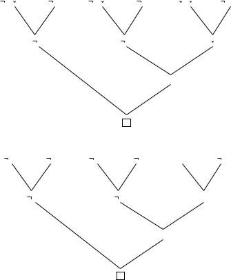
Figure 2.6 Deduction tree 1.

{ H, A}	{ A}	{ C, G}	{ G}	{H, C, M} { M}
{	H}	{	C}	{H, C}
				{H}

Figure 2.7 Deduction tree 2.

Therefore, the clause set is unsatisfiable. Hence the original (unnegated) formula is valid. Figures 2.6 and 2.7 show two versions of a deduction tree corresponding to this deduction.

This resolution theorem forms the basis of most software tools for determining satisfiability of propositional logic formulas. However, the complexity of these tools remains exponential in the original size of the clause set. Chapter 4 presents more efficient representations of boolean formulas using binary decision diagrams (BDDs) that allow faster manipulation of formulas in a number of practical cases. Chapter 6 discusses heuristics for reordering clauses in the decision tree to reduce the search time for determining unsatisfiability.

2.1.2 Predicate Logic

Propositional logic can express simple ideas with no quantitative notions or qualifications, and is also good enough for describing digital logic circuits. For more complex ideas, propositional logic is not sufficient, as shown in the following example.

SYMBOLIC LOGIC

19

Example. Consider the following statements:

Every time the car brake pedal is pressed by the driver of the car, the car stops within 8 seconds. Because Mercedes Benz E320 is a car, whenever the driver of the Mercedes Benz E320 presses its brake pedal, the Mercedes Benz E320 stops within 8 seconds.

Pdenotes “Every time the car brake pedal is pressed by the driver of the car, the car stops within 8 seconds.”

Qdenotes “Mercedes Benz E320 is a car.”

Rdenotes “Whenever the driver of the Mercedes Benz E320 presses its brake pedal, the Mercedes Benz E320 stops within 8 seconds.”

However, R is not a logical consequence of P and Q in the framework of propositional logic.

To handle these statements, we introduce predicate logic, which has the concepts of terms, predicates, and quantifiers. First, we define functions and terms.

Function: A function is a mapping from a list of constants to a constant.

Terms: Terms are defined inductively as follows:

1.Every constant or variable is a term.

2.If f is an n-place function symbol and x1, . . . , xn are terms, then f (x1, . . . , xn ) is a term.

3.All terms are generated using the above rules.

Next, we define predicates and atoms.

Predicate: A predicate is a mapping from a list of constants to either T or F.

Atoms or Atomic Formulas: If P is an n-place predicate symbol and x1, . . . , xn are terms, then P(x1, . . . , xn ) is an atom or atomic formula.

The special symbol is the universal quantifier, and the special symbol is the existential quantifier. If x is a variable, then x means “for all x,” (or “for every x”) and x means “there exists an x.” We also need to define the notions of bound and free variables and variable occurrences.

Bound and Free Variable Occurrences: Given a formula, an occurrence of a variable x is a bound occurrence iff the occurrence is within the scope of a quantifier over this variable or the occurrence immediately follows this quantifier, that is, x appears in a subformula of the form ( x)F or ( x)F. Given a formula, an occurrence of a variable is a free occurrence iff this occurrence is not bound.

20 ANALYSIS AND VERIFICATION OF NON-REAL-TIME SYSTEMS

Often we omit the parentheses surrounding the quantifier and the quantified variable.

Bound and Free Variables: Given a formula, a variable is bound iff at least one occurrence of this variable is bound. Given a formula, a variable is free iff at least one occurrence of this variable is free.

Now we are ready to define formulas in predicate logic.

Well-Formed Formulas: Well-formed formulas in predicate logic are defined recursively as follows:

1.An atom is a formula.

2.If F is a formula, then (¬F) is a formula.

3.If F and G are formulas, then (F op G) is a formula, where op is , , →, or

↔.

4.If F is a formula and x is a free variable in F, then ( x)F and ( x)F are formulas.

5.All formulas are generated using a finite number of the above rules.

Example. Consider the above car example. Let BRAKE STOP signify “Every time the car brake pedal is pressed by the driver of the car, the car stops within 8 seconds.” We have the following predicate logic formulas:

( x)CAR(x) → BRAKE STOP(x))

CAR(MercedesBenzE320).

Since ( x)(CAR(x) → BRAKE STOP(x)) is true for all x, replacing x by “MercedesBenzE320,” we have

(CAR(MercedesBenzE320) → BRAKE STOP(MercedesBenzE320))

is true.

This means that

¬(CAR(MercedesBenzE320) BRAKE STOP(MercedesBenzE320)) is true, but

¬(CAR(MercedesBenzE320)) is false since CAR(MercedesBenzE320) is true.

Therefore, BRAKE STOP(MercedesBenzE320) must be true.

In propositional logic, an interpretation of a formula is an assignment of truth values to the atoms. Since a predicate-logic formula may contain variables, in order to define an interpretation, we need to specify the domain and an assignment to constants, functions symbols, and predicate symbols in the formula.

SYMBOLIC LOGIC

21

Interpretation: An interpretation of a first-order formula F is an assignment of values to each constant, functions symbol, and predicate symbol in F in a nonempty domain D according to the following rules:

1.An element in D is assigned to each constant.

2.A mapping Dn = {(x1, . . . , xn ) | each xi D} to D is assigned to each n-place function symbol.

3.A mapping from Dn to {T,F} is assigned to each n-place predicate symbol.

A formula can be evaluated to true or false given an interpretation over a domain D as follows:

1.The truth values of formulas involving P and Q with logical connectives are evaluated with the table in the previous section on propositional logic.

2.( x)P is T if the truth value of P is evaluated to T for every element in D; else F.

3.( x)P is T if the truth value of P is evaluated to T for at least one element in D; else F.

Example. Suppose we have the following formulas:

( x)IsAutomobile(x) ( x)¬IsAutomobile(x).

An interpretation is:

Domain: D = {MercedesBenzE320, HondaAccord, FordTaurus, Boeing777}.

Assignment:

IsAutomobile(MercedesBenzE320) = T

IsAutomobile(HondaAccord) = T

IsAutomobile(FordTaurus) = T

IsAutomobile(Boeing777) = F

( x)IsAutomobile(x) is F in this interpretation

since IsAutomobile(x) is not T for x = Boeing777. ( x)¬IsAutomobile(x) is T in this interpretation

since ¬IsAutomobile(Boeing777) is T.

Closed Formula: A closed formula has no free occurrences of variables.

22 ANALYSIS AND VERIFICATION OF NON-REAL-TIME SYSTEMS

The definitions for satisfiable formulas and valid formulas are similar to those for propositional logic.

Satisfiable and Unsatisfiable Formulas: A formula G is satisfiable (consistent) iff there is at least one interpretation I in which G is evaluated to T. This interpretation I is said to satisfy G and is a model of G. A formula G is unsatisfiable (inconsistent) iff there is no interpretation I in which G is evaluated to T.

Valid Formula: A formula G is valid iff every interpretation of G satisfies G.

To simplify proof procedures for first-order logic formulas, we first convert these formulas to standard forms discussed next.

Prenex Normal Forms and Skolem Standard Forms We now present a standard form introduced in [Davis and Putnam, 1960] for first-order logic formulas using prenex normal form, conjunctive normal form, and Skolem functions. This form will make it easier to mechanically manipulate and analyze logic formulas. A first-order logic formula can be converted into prenex normal form where all quantifiers are at the left end.

Prenex Normal Form: Formally, a formula F is in prenex normal form iff it is written in the form

(Q1v1) · · · (Qn vn )(M)

where every (Qi vi ), i = 1, . . . , n, is either ( vi ) or ( vi ), and M is a formula with no quantifiers. (Q1v1) · · · (Qn vn ) is the prefix and M is the matrix of F.

The matrix can be converted into a conjunctive normal form (CNF).

The CNF prenex normal form can be converted into a Skolem standard form by removing the existential quantifiers using Skolem functions. This will simplify the proof procedures since existentially quantified formulas hold only for specific values. The absence of existential quantifiers makes it trivially easy to remove the universal quantifiers as well.

Let Qi be an existential quantifier in the prefix (Q1v1) · · · (Qn vn ), 1 ≤ i ≤ n. If there is no universal quantifier to the left of Qi , we replace all vi ’s in the matrix M by a new constant c distinct from the other constants in M, and remove (Qi vi ) from

the prefix.	< u2 · · · < um < i, are universal quantifiers to the
If (Qu1 · · · Qum ), 1 ≤ u1
left of Qi , we replace all vi	in M by a new m-place function f (vu1 , vu2 , . . . , vum )

distinct from those in M and delete (Qi vi ) from the prefix. The resulting formula after removing all existential quantifiers is a Skolem standard form. The constants and functions used to replace the existential quantifiers are called Skolem constants and Skolem functions, respectively.

SYMBOLIC LOGIC

23

Example. Transform the following formula into a standard form:

( x)( y)( z)( u)(P(x, z, u) (Q(x, y) ¬R(x, z))).

We first convert the matrix into a CNF:

( x)( y)( z)( u)((P(x, z, u) Q(x, y)) (P(x, z, u) ¬R(x, z))).

Then we replace the the existential quantifiers with Skolem constants and functions. Starting from the leftmost existential quantifier, we replace its variable x by constant a:

( y)( z)( u)((P(a, z, u) Q(a, y)) (P(a, z, u) ¬R(a, z))).

Next we use a 2-place function f (y, z) to replace the existential variable u:

( y)( z)((P(a, z, f (y, z)) Q(a, y)) (P(a, z, f (y, z)) ¬R(a, z))).

Proving Unsatisfiability of a Clause Set with Herbrand’s Procedure We can view propositional logic as a special case of predicate logic. By treating 0-place predicate symbols as atomic formulas of the propositional logic, predicate logic formulas become propositional logic formulas with no variables, function symbols, and quantifiers. Thus propositional logic formulas can be easily converted into corresponding predicate logic formulas.

However, we cannot in general reduce predicate logic formulas to single formulas of the propositional logic. However, we can systematically reduce a predicate logic formula F to a countable set of formulas without quantifiers or variables. This collection of formulas is the Herbrand expansion of F, denoted by E(F).

A set S of clauses is unsatisfiable iff it is false under all interpretations over all domains. Unfortunately, we cannot explore all interpretations over all domains. However, there is a special domain called the Herbrand universe such that S is unsatisfiable iff S is false under all the interpretations over this domain.

Herbrand Universe: The Herbrand universe of formula F is the set of terms built from the constant a and the function name f , that is, {a, f (a), f ( f (a)), . . .}. More formally, H0 = {a} if there is no constant in the set S of clauses; otherwise, H0 is the set of constants in S. Hi+1, i ≥ 0, is the union of Hi and the set of all terms of the form f n (x1, . . . , xn ), each x j Hi , for all n-place functions f n in S. Hi is the i-level constant set of S, and H∞ is the Herbrand universe of S.

Example. S = {P(x) Q(x), ¬R(y) T (y) ¬T (y)}.

Since there is no constant in S, H0 = {a}. Since there is no function symbol in S,

H = H0 = H1 = · · · = {a}.

24 ANALYSIS AND VERIFICATION OF NON-REAL-TIME SYSTEMS

Ground Instance: Given a set S of clauses, a ground instance of a clause C is a clause obtained by substituting every variable in C by a member of the Herbrand universe H of S.

Atom Set: Let h1, . . . , hn be elements of H . The atom set of S is the set of ground atoms of the form Pn (h1, . . . , hn ) for every n-place predicate in S.

H-Interpretation: An H -interpretation of a set S of clauses is one that satisfies the following conditions:

1.Every constant in S maps to itself.

2.Each n-place function symbol f is assigned a function mapping an element of H n to an element in H , that is, a mapping from (h1, . . . , hn ) to f (h1, . . . , hn ).

Let the atom set A of S be {A1, . . . , An , . . .}. An H -interpretation can be written as a set

I = {e1, . . . , en , . . .}

where ei is either Ai or ¬Ai , i ≥ 1. That ei is Ai means Ai is assigned true; false otherwise.

A set S of clauses is unsatisfiable iff S is false under all the H -interpretations of S. To systematically list all these interpretations, we use semantic trees [Robinson, 1968; Kowalski and Hayes, 1969]. The construction of a semantic tree for S, whether manually or mechanically, is the basis for proving the satisfiability of S. In fact, constructing a semantic tree for S of clauses is equivalent to finding a proof for S.

Semantic Tree: A semantic tree for a set S of clauses is a tree T in which each edge is attached with a finite set of atoms or negated atoms from S such that:

1.There are only finitely many immediate outgoing edges e1, . . . , en from each node v. Suppose Ci is the conjunction of all the literals attached to edge ei . Then the disjunction of these Ci s is a valid propositional formula.

2. Suppose I (v) is the union of all the sets attached to the edges of the branch of T and including v. Then I (v) does not contain any complementary pair of literals (one literal is the negation of the other as in the set {A, ¬A}).

Example. Let the atom set A of S be {A1, . . . , An , . . .}. A complete semantic tree is one in which, for every leaf node L, I (L) contains either Ai or ¬Ai , where i =

1, 2, . . . .

A node N in a semantic tree is a failure node if I (N ) falsifies a ground instance of a clause in S, and for each ancestor node N of N , I (N ) does not falsify any ground instance of a clause in S.

SYMBOLIC LOGIC

25

Closed Semantic Tree: A closed semantic tree is one in which every branch ends at a failure node.

Herbrand’s Theorem (Using Semantic Trees): A set S of clauses is unsatisfiable iff a corresponding finite closed semantic tree exists for every complete semantic tree of S.

Herbrand’s Theorem: A set S of clauses is unsatisfiable iff a finite unsatisfiable set S of ground instances of clauses of S exists.

Given an unsatisfiable set S, if a mechanical procedure can incrementally generate sets S1 , S2 , . . . and check each Si for unsatisfiability, then it can find a finite number n such that Sn is unsatisfiable.

Gilmore’s computer program [Gilmore, 1960] followed this strategy of generating the Si s, replacing the variables in S by the constants in the i-level constant set Hi of S. It then used the multiplication method (for deriving the empty clause ) in the propositional logic to test the unsatisfiability of each Si since it is a conjunction of ground clauses (with no quantifiers).

Proving Unsatisfiability of a Clause Set Using the Resolution Procedure

The above proof technique based on Herbrand’s theorem has a major shortcoming in that it requires the generation of sets of ground instances of clauses, and the number of elements in these sets grows exponentially. We now present the resolution principle [Robinson, 1965], which can be applied to any set of clauses (whether ground or not) to test its unsatisfiability. We need several additional definitions.

Substitution: A substitution is a finite set of the form {t1/v1, . . . , tn /vn } where the vi s are distinct variables and the ti s are terms different from the vi s. Here, there are n substitution components. Each vi is to be replaced by the corresponding ti . The substitution is a ground substitution if the ti s are ground terms. Greek letters are used to denote substitutions.

Example. θ1 = {a/y} is a substitution with one component. θ2 = {a/y, f (x)/x, g( f (b))/z} is a substitution with three components.

Variant: A variant (also called a copy or instance), denoted Cθ, of a clause C is any clause obtained from C by a one-to-one replacement of variables specified by the substitution θ. In other words, a variant C can be either C itself or C with its variables renamed.

Example. Continuing the above example, let C = (¬(R(x) O(y)) D(x, y)). Then Cθ1 = ¬(R(x) O(a)) D(x, a).

26 ANALYSIS AND VERIFICATION OF NON-REAL-TIME SYSTEMS

Unification Algorithm:

(1)i := 0, ρi := , Ci := C.

(2)If |Ci | = 1, C is unifiable and return ρi as a most general unifier for C. Else, find the disagreement set Di of Ci .

(3)If there are elements xi , yi Di such that xi does not appear in yi , go to step (4). Else, return “C is not unifiable.”

(4) ρi+1 := ρi {yi /xi }, Ci+1 := Ci {yi /xi }, i := i + 1, go to step (2). Observe that

Ci+1 = Cρi+1.

Figure 2.8 Unification algorithm.

Separating Substitutions: A pair of substitutions θ1 and θ2 for a pair of clauses C1 and C2 is called separating if C1θ1 is a variant of C1, C2θ2 is a variant of C2, and C1θ1 and C2θ2 have no common variable.

Unifier: A substitution θ is a unifier for a set C = {C1, . . . , Cn } of expressions iff C1θ = · · · = Cn θ. A set C is unifiable if it has a unifier. A unifier for set C is a most general unifier (MGU) iff there is a substitution λ such that ρ = θ ◦ λ for every unifier ρ for set C.

Example. Let S = {P(a, x, z), P(y, f (b), g(c))}. Since the substitution θ = {a/y, f (b)/x, g(c)/z} is a unifier for S, S is unifiable.

Unification Theorem: Any clause or set of expressions has a most general unifier.

Now we are ready to describe an algorithm for finding a most general unifier for a finite set C of nonempty expressions (Figure 2.8). The algorithm also determines if the set is not unifiable.

Resolvent: Let C1 and C2 be two clauses with no common variable and with separating substitutions θ1 and θ2, respectively. Let B1 and B2 be two nonempty subsets (literals) B1 C1 and B2 C2 such that B1θ1 and ¬B2θ2 have a most general unifier ρ. Then the clause ((C1 − B1) (C2 − B2))ρ is the binary resolvent of C1 and C2, and the clause ((C1 − B1)θ1 (C2 − B2)θ2)ρ is the resolvent of C1 and C2.

Given a set S of clauses, R(S) contains S and all resolvents of clauses in S, that

is, R(S) = S {T : T is a resolvent of two clauses in S}. For each i ≥ 0, R0(S) = S,

Ri+1(S) = R(Ri (S)), and R (S) = {Ri (S)|i ≥ 0}.

Example

Let C1 = ¬A(x) O(x) and C2 = ¬O(a). A resolvent of C1 and C2 is ¬A(a). Let C3 = ¬R(x) ¬O(a) D(x, a) and C4 = R(b). A resolvent of C3 and C4 is ¬O(a) D(b, a).

SYMBOLIC LOGIC

27

We are ready to present the resolution theorem for predicate logic.

Resolution Theorem: A clause set S is unsatisfiable iff there is a deduction of the empty clause from S, that is, R (S).

The resolution theorem and the unification algorithm form the basis of most computer implementations for testing the satisfiability of predicate logic formulas. Resolution is complete, so it always generates the empty clause from an unsatisfiable formula (clause set).

Example. Consider the premise and the conclusion in English. The premise is: Airplanes are objects. Missiles are objects. Radars can detect objects. The conclusion is: Radars can detect airplanes or missiles. We want to prove the premise implies the conclusion.

Let A(x) denote “x is an airplane,” M(x) denote “x is a missile,” O(x) denote “x is an object,” R(x) denote “x is a radar,” D(x, y) denote “x can detect y.” We are ready to represent the premise and conclusion as predicate logic formulas.

Premise:

( x)(A(x) → O(x)) ( x)(M(x) → O(x))

( x)( y)(R(x) O(y) → D(x, y)).

Conclusion: ( x)( y)(R(x) (A(y) M(y)) → D(x, y)).

Then we negate the conclusion. Next we convert these formulas into prenex normal form and then CNF.

Premise:

1.¬A(x) O(x)

2.¬M(x) O(x)

3.y(¬(R(x) O(y)) D(x, y))

=¬(R(x) O(a)) D(x, a)

=¬R(x) ¬O(a) D(x, a).

Negation of conclusion:

¬( x)( y)(R(x) (A(y) M(y)) → D(x, y))

=( x)( y)¬(¬(R(x) (A(y) M(y))) D(x, y))

=( x)(R(x) (A(y) M(y)) ¬D(x, y))

=R(b) (A(y) M(y)) ¬D(b, y).

Therefore, we have three clauses