translation - 2.18

2.2.5 Damping and Drag

A damper is a component that resists motion. The resistive force is relative to the rate of displacement. As mentioned before, springs store energy in a system but dampers dissipate energy. Dampers and springs are often used to compliment each other in designs.

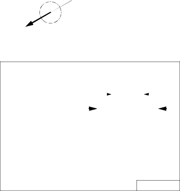
Damping can occur naturally in a system, or can be added by design. The physical damper pictured in Figure 2.18 uses a cylinder that contains a fluid. There is a moving rod and piston that can slide within the cylinder. As the piston moves, fluid is forced through a small orifice. When moved slowly the fluid moves easily, but when moved quickly the pressure required to force the fluid through the orifice rises. This rise in pressure results in a higher force of resistance. In ideal terms any motion would result in an opposing force. In reality there is also a break-away force that needs to be applied before motion begins. Other manufacturing variations could also lead to other small differences between dampers. Normally these cause negligible effects.

orifice
	motion
fluid	fluid
piston

Figure 2.18 A physical damper

The basic equation for an ideal damper in compression is shown in Figure 2.19. In this case the force and displacement are both compressive. The force is calculated by multiplying the damping coefficient by the velocity, or first derivative of position. Aside from the use of the first derivative of position, the analysis of dampers in systems is similar to that of springs.

translation - 2.19

x

Kd

d

(15)

F

= K

----

x

F

d dt

Aside: The symbol shown is typically used for dampers. It is based on an old damper design called a dashpot. It was constructed using a small piston inside a larger pot filled with oil.

Figure 2.19 An ideal damper

Damping can also occur when there is relative motion between two objects. If the objects are lubricated with a viscous fluid (e.g., oil) then there will be a damping effect. In the example in Figure 2.20 two objects are shown with viscous friction (damping) between them. When the system is broken into free body diagrams the forces are shown to be a function of the relative velocities between the blocks.

x1

( x·

– x·

)

F

= K

Kd

d

d

1

2

( x·

– x· )

F

d

= K

d

1

2

x2

Aside: Fluids, such as oils, have a significant viscosity. When these materials are put in shear they resist the motion. The higher the shear rate, the greater the resistance to flow. Normally these forces are small, except at high velocities.

Figure 2.20 Viscous damping between two bodies with relative motion

A damping force is proportional to the first derivative of position (velocity). Aerodynamic drag is proportional to the velocity squared. The equation for drag is shown in

translation - 2.20

Figure 2.21 in vector and scalar forms. The drag force increases as the square of velocity. Normally, the magnitude of the drag force coefficient ’D’ is approximated theoretically and/or measured experimentally. The drag coefficient is a function of material type, surface properties, object size and object geometry.

v

F

F = –D

v

v

Figure 2.21 Aerodynamic drag

The force is acting on the cylinder, resulting in the velocities given below. What is the applied force?

d

m

d

m

----x

1

= 0.1---

----x

2

= –0.3---

dt

s

dt

s

F

F

k

Ns

d

= 0.1------

m

ans. F = –0.02N

Figure 2.22 Drill problem: Find the required forces on the damper

translation - 2.21

2.2.6 Cables And Pulleys

Cables are useful when transmitting tensile forces or displacements. The centerline of the cable becomes the centerline for the force. And, if the force becomes compressive, the cable becomes limp, and will not transmit force. A cable by itself can be represented as a force vector. When used in combination with pulleys, a cable can redirect a force vector or multiply a force.

Typically we assume that a pulley is massless and frictionless (in the rotation chapter we will assume they are not). If this is the case then the tension in the cable on both sides of the pulley are equal, as shown in Figure 2.23.

T1

for a massless frictionless pulley

T1 = T2

T2

Figure 2.23 Tension in a cable over a massless frictionless pulley

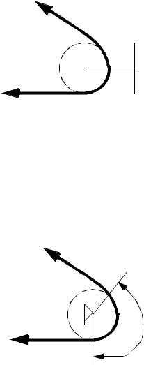
If we have a pulley that is fixed and cannot rotate, the cable must slide over the surface of the pulley. In this case we can use the coefficient of friction to determine the relative ratio of forces between the sides of the pulley, as shown in Figure 2.24.

T1

T2	µ	k ( ∆θ )
-----	= e
T1

∆θ

T2

Figure 2.24 Friction of a belt over a fixed drum

translation - 2.22

Given,

s = 0.35 k = 0.2

M = 1Kg

Find F to start the mass moving up and down, and then the force required to maintain a low velocity motion.

M
						F
ans.				0.2				π
Fup		= 9.81e						2
									N
F			=	9.81N
	down			--------------
				0.2		π
						--
				e		2

Figure 2.25 Drill problem: Friction forces for belts on drums

Although the discussion in this section has focused on cables and pulleys, the theory also applies to belts over drums.