Karimi A.PID controller tuning using Bode's integrals

812	IEEE TRANSACTIONS ON CONTROL SYSTEMS TECHNOLOGY, VOL. 11, NO. 6, NOVEMBER 2003

PID Controller Tuning Using Bode’s Integrals

Alireza Karimi, Daniel Garcia, and Roland Longchamp

Abstract— A new method for PID controller tuning based on Bode’s integrals is proposed. It is shown that the derivatives of amplitude and phase of a plant model with respect to frequency can be approximated by Bode’s integrals without any model of the plant. This information can be used to design a PID controller for slope adjustment of the Nyquist diagram and improve the closed-loop performance. Besides, the derivatives can be also employed to estimate the gradient and the Hessian of a frequency criterion in an iterative PID controller tuning method. The frequency criterion is defined as the sum of squared errors between the desired and measured gain margin, phase margin and crossover frequency. The method benefits from specific feedback relay tests to determine the gain margin, the phase margin and the crossover frequency of the closed-loop system. Simulation examples and experimental results illustrate the effectiveness and the simplicity of the proposed method to design and tune the PID controllers.

Index Terms— Autotuning, iterative methods, proportional control, relay control system, robustness.

I. INTRODUCTION

PID controllers are widely used in industrial plants and different methods for the design or the tuning of these controllers have been proposed in the literature [1]–[3]. The available methods are normally based on a first or a second-order model with time delay obtained from the time response or the measurement of multiple points on the frequency response of the process. The specifications are often expressed in terms of phase and/or gain margins [4]–[6], because they are the classical measures of robustness and together with the crossover frequency, they represent the time domain performance of the closed-loop system as well. This problem, in general, even if the plant model is perfectly known, leads to a set of nonlinear equations for which no analytic solution is available. The traditional methods are the graphical algorithms using Bode plots which are not very suitable for autotuning of the PID controllers. More advanced methods try either to find a solution by numerical methods [5] or to simplify the equations using some approximations to find an analytic solution [6]. The main drawback of these approaches is that the desired specifications are not necessarily achieved on the real system because of the approximations in modeling and/or equations. In addition, they do not lead to on-line tuning methods in order to meet the specifications for

the real plant.

In 1984, Åström and Hägglund [4] proposed an automatic tuning method based on a simple relay feedback test which gives, using the describing function analysis, the critical gain and the critical frequency of the system. Other points on the Nyquist curve can be identified using a relay with hysteresis [4] or by introducing an adjustable time delay in the closed-loop system [7], [8]. A closed-loop relay test scheme was proposed in [9] which identifies directly the crossover frequency (the frequency at which the loop gain is equal to 1). After identifying a point on the frequency response of the plant, the so-called modified Ziegler–Nichols method can be used to move this point to another position in the complex plane [1]. Two equations for phase and amplitude assignment are obtained which can be solved to find the parameters of a PI or PD controller. For a PID controller, however, an additional equation should be introduced. In the modified Ziegler–Nichols method, the ratio between integral time

Manuscript received February 12, 2002. Manuscript received in final form April 2, 2003. Recommended by Associate Editor D. W. Repperger. This work was supported by the Swiss National Science Foundation by Grant 2100-064931.01.

The authors are with the Laboratoire d’Automatique, Ecole Polytechnique Fédérale de Lausanne (EPFL), 1015 Lausanne, Switzerland (e-mail: [e-mail]).

Digital Object Identifier 10.1109/TCST.2003.815541

KARIMI et al.: PID CONTROLLER TUNING USING BODE’S INTEGRALS

813

and the relay output amplitude. Then the phase of the identified point can be computed as follows:

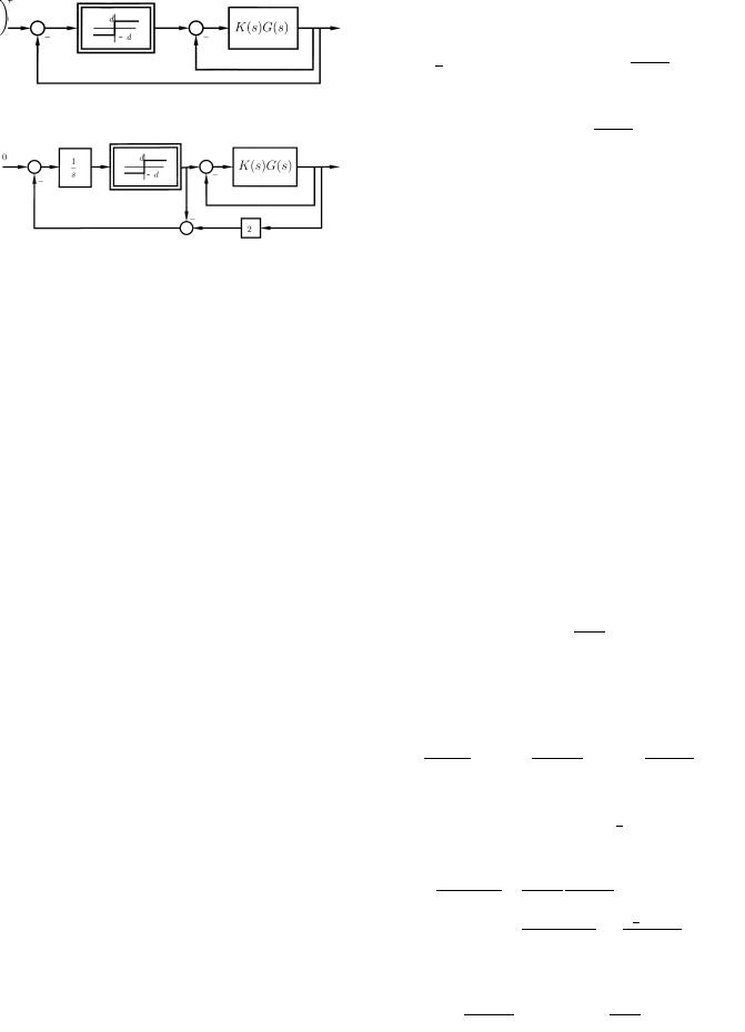
Fig. 1. Relay experiment for gain margin measurement.

Fig. 2. Relay experiment for phase margin mesurement.

An iterative procedure for gain and phase margin adjustment for a PI controller was presented in [12]. The approach uses similar relay tests, but the gradient of the criterion is not calculated and an ad hoc algorithm is used, instead. As a result the algorithm converges much slower than the proposed method.

The paper is organized as follows: In Section II several relay feedback tests will be briefly reviewed. Section III shows how the Bode’s integrals can be employed for slope adjustment in the modified Ziegler–Nichols method. An iterative tuning method for gain and phase margin adjustment together with simulation examples are presented in Section IV. An application of the proposed method to a three-tank system in Section V shows the effectiveness and fast convergence of the iterative method. Finally, Section VI gives some concluding remarks.

II. RELAY FEEDBACK TEST

The relay method is a well-known technique to identify useful points on the Nyquist curve by generating an appropriate oscillation with a relay feedback. In the standard relay method the controller is replaced by an on-off relay in closed-loop. For many systems there will be an oscillation when the control signal is a square wave and the process output is close to a sinusoid. The amplitude and the frequency of the limit cycle obtained give, respectively, the point where the Nyquist curve intersects the negative real axis and its corresponding frequency.

Relay feedback can also be applied to closed-loop systems including a linear controller. Fig. 1 shows an experiment where the relay output is the reference signal for the closed-loop system with an existing controller and the closed-loop output is fed back to the relay input. The identified point, obtained from the amplitude of the limit cycle, is on the intersection of the open-loop Nyquist curve with the segment ( 1,0). The gain margin is defined as the inverse of the amplitude of the identified point.

The experiment proposed in [9] and shown in Fig. 2 generates a limit cycle at the crossover frequency of the open-loop transfer function . The phase margin can be approximated by the amplitude and frequency of the generated limit cycle [13]. Let be the measured limit cycle frequency (equal to the crossover frequency), the relay input amplitude

The phase margin is then given by

The proposed methods for measuring the gain and phase margins by the relay method have the drawback that the method of the describing function must be used for the identification of the frequencies and the points on the Nyquist curve of interest. This approach is approximative. Several methods are proposed to improve the precision of the approximations [2]. In this paper, an adaptive identification method to the critical gain proposed in [14] is used in all of the simulation examples and experiments. In this method the relay is replaced by a saturation nonlinearity and a time varying gain.

III. LOOP SLOPE ADJUSTMENT USING BODE’S INTEGRALS

The slope of the Nyquist curve at the crossover frequency affects drastically the performance and robustness of the closed-loop system. In this section, first a formula is derived which gives the relation between and for obtaining the desired slope of the Nyquist curve of the loop transfer function at a given frequency. Then the Bode’s integrals are used to approximate the derivatives of the plant transfer function. Finally, the parameters of a PID controller for the desired phase margin and slope at a given frequency are determined.

A. Loop Slope Adjustment

Consider the loop transfer function where

(1)

is the PID controller. The slope of the Nyquist curve of the loop transfer function at defined by is equal to the phase of the derivative of at . The derivative of the loop transfer function with respect to is computed as follows:

(2)

Furthermore, one has

(3)

Differentiating this equation gives

(4)

On the other hand, the derivative of the controller with respect to is

(5)

814 IEEE TRANSACTIONS ON CONTROL SYSTEMS TECHNOLOGY, VOL. 11, NO. 6, NOVEMBER 2003

Substituting (1), (4) and (5) into (2), one obtains

(the slope of the Bode plot) near . There-

fore, assuming that the slope of the Bode plot is almost constant

in the neighborhood of ,

can be approximated by:

(6)

Hence, the slope of the Nyquist curve at is given by

(7)

where and and are defined as follows:

(8)

(9)

It is desired to adjust the slope of the Nyquist curve of the loop transfer function to a specified value . Then straightforward calculation gives

(10)

In the next part, and are directly approximated using the Bode’s integrals.

B. Bode’s Integrals

The relations between the phase and the amplitude of a stable minimum-phase system have been investigated for the first time by Bode [11]. The results are based on Cauchy’s residue theorem and have been extensively used in network analysis. Two integrals are presented in this section. The first one, which is well known in the control engineering field, shows the relationship between the phase of the system at each frequency as a function of the derivative of its amplitude. But the second integral, to the best of the authors’ knowledge, has never been used in control design. The integral shows how the amplitude of the system at each frequency is related to the derivative of the phase and the static gain of the system.

1) Derivative of Amplitude: Bode has shown in [11] that for a stable minimum-phase transfer function , the phase of the system at is given by:

										(11)
where					. Since			decreases rapidly
as	deviates from , the						integral depends mostly on

(12)

This property is often used in loop shaping where the slope of the amplitude Bode plot at the crossover frequency is limited to 20 dB/decade in order to obtain approximately a phase margin of 90 . Here the measured phase of the system at is used to determine approximately the slope of the amplitude Bode plot

:

(13)

2) Derivative of Phase: The second Bode’s integral shows that the amplitude of a stable minimum-phase system can be determined uniquely from its phase and its static gain. More precisely, the logarithm of the system amplitude at is given by [11]

(14) where is the static gain of the plant. In the same way, assuming that is linear (in a logarithmic scale) in the neighborhood of , one has

which gives

(15)

Note that for the systems containing an integrator, the static gain cannot be computed. For such systems, the static gain of the system without the integrator should be estimated and used in the above formula (note that the phase of the integrator is constant and its derivative is zero).

3) Precision of the Estimates: The precision of the estimates of the derivatives of amplitude and phase depends on the system dynamics and on the frequency at which the experiments are performed. However, extensive simulations on the typical models of industrial plants have shown that the absolute normalized error of the estimates is in an acceptable range. In

KARIMI et al.: PID CONTROLLER TUNING USING BODE’S INTEGRALS

815

4) Effect of Pure Time Delay: Consider the following system with a pure time delay :

(17)

where is a stable minimum-phase system. Differentiating the amplitude and phase of with respect to gives

(18)

(19)

Now using the Bode’s integral from (12), the phase of at is approximated by

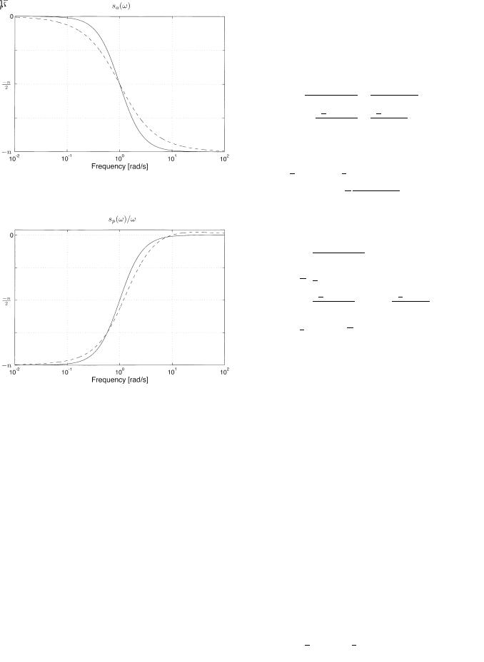
Fig. 3. Comparison of true s (!) and the estimated one based on Bode’s integral (solid line: true values, dashed line: estimates).

(20)

Then and for a system including a pure time delay are computed as follows:

(21)

Fig. 4. Comparison of true s (!)=! an dthe based on Bode’s integral (solid line: true values, dashed line: estimates).

order to give an idea about the precision of the estimates, let us consider the following system

			(16)
where is a positive integer. The true values of			and

computed on the basis of the model for different frequencies, are compared with the estimated ones based on the Bode’s integrals in Fig. 3 and Fig. 4, respectively. It can be observed that the maximum of the absolute normalized error does not exceed 0.1 for this system.

Similar results can be obtained for the systems presented by several first-order models in cascade. For oscillatory systems, the estimation may be poor at certain frequencies, but in general the results remain satisfactory. For nonminimum-phase systems the Bode’s integrals are no longer valid and the proposed formulas give incorrect results. However, it will be shown next that the pure time delay has no effect on the estimation of and its effect on the estimation of can be neglected if it is small with respect to the dominant time constant of the system.

(22) The above relations show that the pure time delay should be

known for the calculation of		but it has no effect on the
calculation of	. It should be remembered that represents

the pure time delay of the system which is usually related to the mass transport delay and is often negligible or can be easily measured. This value should not be confounded with the time delay that is used to model a high-order system as a firstor second-order system with delay. For example, has no pure time delay whereas it can be approximated by a first-order model with a large time delay.

C. PID Design

Suppose that the amplitude and the phase of a plant at the crossover frequency are known. These values may be obtained using the existing controller and by the method mentioned in Section II. Suppose also that the static gain of the process is measured. The objective is to improve the controller performance by adjusting the phase margin and the slope of the Nyquist curve at the crossover frequency. The modified Ziegler–Nichols method is used but the derivatives are approximated by the Bode’s integrals, so no model for the system is required. To obtain a desired phase margin at the crossover frequency we have the following equations to solve

(23)

(24)

816	IEEE TRANSACTIONS ON CONTROL SYSTEMS TECHNOLOGY, VOL. 11, NO. 6, NOVEMBER 2003

Solving these equations one obtains

(25)

(26)

where is the phase of . Now we exploit (10) in order to obtain the desired slope at the crossover frequency. Combining (10) and (26), we obtain after straightforward calculations the parameters and as follows:

(27)

(28)

The improved PID controller is now defined by (25), (27), and (28).

D. Example

The PID design method presented above will be illustrated by the following simulation model

(29)

The specifications are set at 0.4 rad/s for the crossover frequency and 50 for the phase margin. First, the control parameters are obtained using the modified Ziegler–Nichols method. The resulting PID controller is

			(30)
This controller moves the point			of the Nyquist curve
to a point of	on the unit circle having a phase of

130 . This conforms to the closed-loop system with the specifications mentioned above.

In order to improve the closed-loop performance, let us calculate now a controller that provides the closed-loop system the same crossover frequency and phase margin, but with the desired slope of the open-loop Nyquist curve at the crossover frequency of 65 . This reduces the current slope of the Nyquist curve by 25 and ensures a greater distance of the Nyquist curve from the critical point in high frequencies. The controller parameters are obtained from (25), (27), and (28), where

and	are approximated using (13) and (15)
			(31)

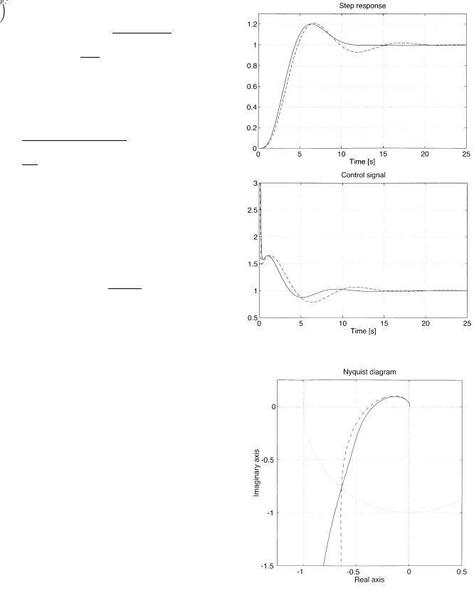
Although the approximation error for and leads to a resultant slope of 74 (about 13% error), a comparison of the closed-loop performance for the two controllers shown in Fig. 5 illustrates a significant improvement of the closed-loop performance. The overshoot is about the same but the settling time is 44% smaller with the proposed method. It should be mentioned that, in simulation, the derivative part of the ideal PID controller

Fig. 5. Step response of the closed-loop system (dashed line: modified Ziegler-Nicholas, solid line: proposed).

Fig. 6. Nyquist diagram (dashed line: modified Ziegler–Nichols, solid line: proposed).

is replaced by a causal derivator and no saturation is considered for the control signal. The Nyquist diagrams (Fig. 6) further show that the proposed controller modifies the slope of the Nyquist curve and as a result improves the gain

KARIMI et al.: PID CONTROLLER TUNING USING BODE’S INTEGRALS

817

margin as well as the modulus margin (the minimum distance between and the critical point) of the system.

IV. ITERATIVE PID TUNING IN CLOSED-LOOP

In the previous section, it was assumed that the amplitude and the phase of the plant at the crossover frequency are known or they are measured by a relay feedback experiment with an existing controller. However, if the desired crossover frequency is different from the measured one, an analytic solution as presented in the previous section cannot be obtained. Therefore it is not possible, for example, to improve the performance of the closed-loop system by increasing the crossover frequency which is closely related to closed-loop bandwidth. In addition, although the Nyquist curve of the loop transfer function passes through a point with the desired phase, it is not guaranteed that this point gives the phase margin (it is possible that the Nyquist curve intersects several times the unit circle). So an extra relay feedback test using the new controller should be carried out in order to validate the desired performance on the real system.

In this section, an iterative tuning method in the frequency domain is proposed. The method is based on the measurement of the phase margin and the crossover frequency by the closed-loop relay test of Section II improved by an adaptive gain adjustment proposed in [14]. In this method, a frequency criterion is minimized iteratively using the Gauss–Newton algorithm. The particularity of this method is that the gradient of the criterion is approximated using the Bode’s integrals and no model of the plant is required.

A. Iterative Procedure for Phase Margin Adjustment

only and and (10) is used at each iteration to compute

.

The gradient of the criterion is given by

(34)

where is the derivative of the phase margin with respect to computed through the chain rule (note that is a function

of and )

(35)

Now replacing in the above equation by gives

(36)

The first term in the above equation is equal to which is completely known at each iteration. Furthermore one has

(37)

Again, the first term is completely known and can be approximated using (15). Now, it only remains to compute . For this purpose, we use the fact that the loop gain at in each iteration is equal to 1, therefore its derivative (or derivative of its logarithm) with respect to will be zero. Then one has

First of all, a performance criterion in the frequency domain

is defined as follows:

(38)

(32)

but from the Bode’s integral (see (13)) one has

(39)

where

is the vector of the controller parameters, and are,

respectively, the measured and desired crossover frequencies,

Thus,

can be approximated as follows (note that

and

and are the measured and desired phase margins.

)

The error between the measured and the desired values are nor-

malized in order to avoid numerical problems in the iterative al-

(40)

gorithm. In the next step, the controller parameters minimizing

the criterion are obtained by the iterative Newton formula

Notice that the gradient of the criterion is computed using only

(33)

the measured crossover frequency and the measured ampli-

tude and phase of the plant. In the same way, the Hessian of the

where

is the iteration number,

is a positive scalar repre-

criterion can be approximated without any additional informa-

tion as follows:

senting the step size,

is a square positive definite matrix of

dimension , and

is the gradient of the criterion with re-

spect to

. This algorithm converges to the vector of parameters

minimizing the criterion, provided that the step size is properly

chosen [15]. The matrix

can be chosen equal to the identity

(41)

matrix or to the Hessian of the criterion to obtain faster conver-

gence (Gauss–Newton method).

The last two terms can be neglected because they are small espe-

It should be mentioned that the slope of the loop Nyquist

cially in the neighborhood of the final solution. In addition, this

curve can also be adjusted simultaneously in the iterative ap-

simplification makes the Hessian always positive which fixes

proach. In fact, in this case, the vector of parameters contains

the numerical problems normally encountered in the iterative

818	IEEE TRANSACTIONS ON CONTROL SYSTEMS TECHNOLOGY, VOL. 11, NO. 6, NOVEMBER 2003

Newton algorithm. The use of the Hessian matrix in the iterative formula (33) instead of significantly improves the convergence speed.

(42)

B. Iterative Procedure for Phase and Gain Margins Adjustment

In phase margin and slope adjustment procedures, the controller is designed using only the information on one frequency point of the plant. Although this approach is very fast and simple and works well for the majority of the industrial processes, it may not work appropriately for some complex high-order systems. This means that the specifications may be satisfied just locally at the crossover frequency and it is possible that the behavior of the system changes drastically elsewhere, leading, for example, to a very small gain margin. For such systems, it may be preferable to tune the phase and gain margins at the same time. However, this necessitates two relay experiments in each iteration: one relay test to measure the gain margin and the other for the phase margin. A frequency criterion can be defined as follows:

	(43)
where	is the amplitude of the loop transfer
function where it intersects the negative real axis
.	is the critical loop frequency, is the inverse of the

desired gain margin. The gradient of the criterion is given by

(44)

where is the derivative of the critical loop gain with respect to computed as follows:

(45)

The first term is equal to which can be easily computed at each iteration. The second term can be approximated using the Bode’s integrals in a similar way as is done for the phase margin. First the derivative of the amplitude of the loop gain is computed using (13) as follows:

(46)

The first term in the above equation is equal to which can be computed knowing the controller at each iteration. Furthermore, one has

(48)

Again, knowing the controller at each iteration, the first term in the right-hand side (RHS) can be computed while the second term is approximated using the Bode’s integral of (15). Therefore, is given by

(49)

In a similar way an approximation of the Hessian can also be computed as follows:

(50)

C. Simulation Example

Now let us consider a complex plant model including a time delay as follows:

(51)

This model was proposed in [16] and represents a difficult problem to be solved using a PID controller. It should be noted that neither the traditional Ziegler–Nichols method nor a more advanced method based on a first-order plant model [6] can give a stabilizing controller for this plant. Contrary to the simulation example presented in Section III-D, it is very difficult here to tune a controller using the slope adjustment method, because a small change in the slope of the Nyquist curve at the crossover frequency may even make the closed-loop system unstable. In the following, it is shown that a controller which confers appropriate specifications on the closed-loop system can be tuned with the iterative phase and gain margins adjustment method. This method requires two experiments per iteration and is more convenient for high-order complex systems. However, one should note that the experimental time for the gain margin measurement can be chosen to be smaller than that of the phase margin, because the critical frequency is appreciably larger than the crossover frequency.

The specifications are set for this example at

for the crossover frequency, and and for the phase and for the inverse of the gain margin, respectively. The initial controller is designed using the Kappa-Tau tuning rule proposed in [1], which gives the following stabilizing controller

Then	is computed using the fact that in each iteration		(52)

and consequently its derivative with respect to

will be zero, which gives											The performance criterion of (43) is considered. Two
											closed-loop experiments are performed to measure a crossover
										(47)	frequency of 0.139 rad/s, a phase margin of 78.5 and a gain
											margin of 4.39, which give a performance criterion of 0.104.

KARIMI et al.: PID CONTROLLER TUNING USING BODE’S INTEGRALS

819

Fig. 8. Schematic diagram of the tank system.

Fig. 7. Step response of the closed-loop system (dashed line: Kappa-Tau; solid line: proposed).

With these values, the gradient and Hessian are calculated, and a new controller is obtained. After one other iteration the following controller is obtained

(53)

with a performance criterion of 0.0017. This controller gives 0.1997 rad/s for the crossover frequency, 66.0 for the phase margin and 2.97 for the gain margin. It should be noted that no significant improvement can be achieved with further iterations. A comparison of the closed-loop performance between the initial controller and the final one in Fig. 7 shows that a much smaller settling time is achieved with an overshoot of only 0.7%. In the simulation example, is replaced by a causal derivator .

It is worth mentioning that even if the estimation errors of might be large due to the presence of an unknown pure time delay in the plant model, the criterion converges rapidly enough. The reason is that in the Gauss-Newton algorithm the quadratic criterion will converge to its minimum value even with an ap-

proximative gradient.

V. REAL-TIME EXPERIMENT

In this section, experimental results obtained with a three-tank system (Fig. 8) are presented. The process consists

of three cylinders T1, T2, and T3 which are interconnected in series by two connecting pipes. Two pumps, driven by dc motors, supply the tanks T1 and T2 with the liquid (water) collected in a reservoir. The water level in each tank is measured by a piezoresistive pressure transducer. The first tank is equipped with a manually adjustable valve which lets the water

outflow at rate	to the reservoir. The input of the process
is an electrical signal which controls the flow rate			into the
first tank. The output		of the process is the voltage of the

piezoresistive pressure transducer of T2, which is proportional to the level with a negative gain. The second pump acts as an output disturbance to the system. The control objective is to maintain the level of T2 at a desired value. Due to nonlinear

relations between the input flow rate			, the output flow rate
	and the tank level, the system is nonlinear.
	Consider that the system operates at a set point corresponding
to	, where	is the maximum flow rate

of the pump. For this operating point, an initial controller is designed using the Kappa-Tau tuning rule proposed in [1] based on the step response of the system. The resulting PID controller is

(54)

It should be noted that the Ziegler–Nichols method gives an unstable controller for this operating point. After measuring a static gain of about 1, a closed-loop experiment as proposed in Section II identifies for this configuration a phase margin of 64 and a crossover frequency of 0.097 rad/s. In order to improve the stability of the closed-loop system and reduce the control effort, new specifications with an increased phase margin and a reduced crossover frequency compared with the actual ones, are defined , . As another specification, a desired value for the slope of the Nyquist curve at crossover frequency or a constant ratio between the integral time and the derivative time should be considered. In this experiment, like in the classical Ziegler–Nichols, is considered and the derivative part of the controller is replaced by a causal derivator . In the next step, the gradient

820	IEEE TRANSACTIONS ON CONTROL SYSTEMS TECHNOLOGY, VOL. 11, NO. 6, NOVEMBER 2003

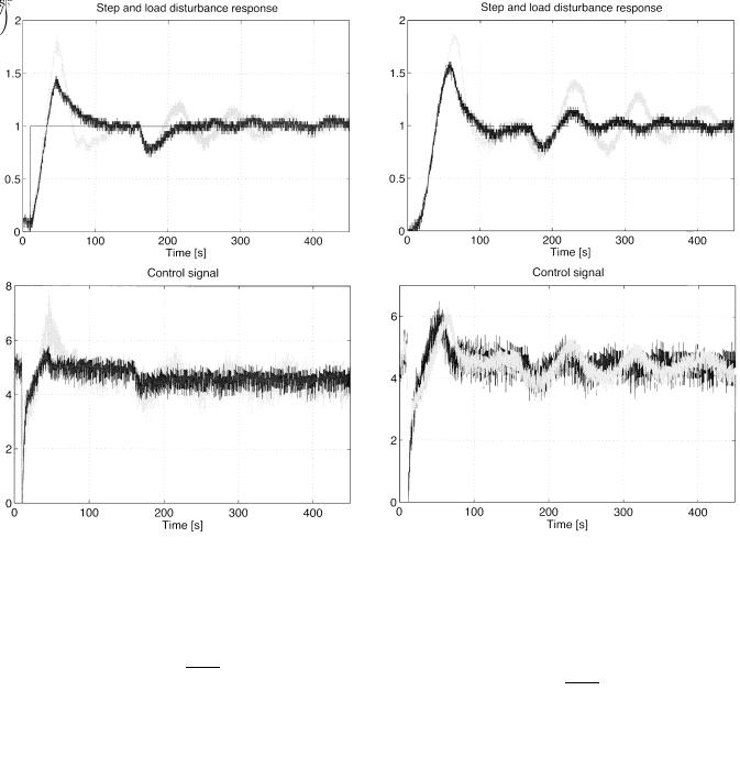
Fig. 9. Normalized step and disturbance response of the closed-loop system (grey line: Kappa-Tau. black line: proposed).

Fig. 10. Normalized step and disturbance response of the closed-loop system (grey line: controller (55). black line: controller (56)).

and the Hessian are calculated and a new controller is obtained after the first iteration

(55)

The closed-loop test applied to the system with the controller in (55) gives the following estimates

As the estimated values are close to the desired ones, there is no need for further iterations. A comparison between the time response of the closed-loop system with the Kappa-Tau controller and the proposed one is shown in Fig. 9. The step response is normalized and the output disturbance concerns a constant flow rate for the pump 2 applied at . It can be seen that the proposed controller gives a much better performance for the closed-loop system in terms of disturbance rejection, overshoot and settling time.

Now, consider that the operating point of the system is changed and, due to the system nonlinearity, the closed-loop performance deteriorates. Consequently, the same controller at the new operating point does not meet the specification (a phase margin of and a crossover frequency of 0.066

rad/s are obtained) and the controller should be retuned. After one iteration, using the proposed tuning method, the following controller is obtained

(56)

The closed-loop system with this controller gives the following performance which is very close to the desired one

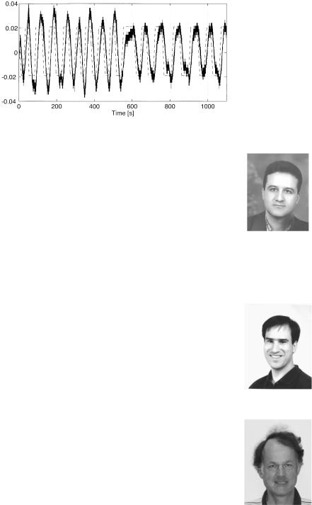
A comparison of the normalized step response and disturbance response of the closed-loop system with the two controllers is shown in Fig. 10. The effectiveness and rapidity of the proposed algorithm is shown in Fig. 11 for an autotuning experiment. During the first 500 s the initial controller is implemented on the real system and measurements are performed. Then the controller is updated and a new test is carried out for measuring the phase margin as well as the crossover frequency.

As shown in this section, the proposed iterative tuning algorithm is fast enough to be used for the autotuning of real processes, and is particularly appropriate for readjusting the controller parameters of systems whose operating point changes slowly.

KARIMI et al.: PID CONTROLLER TUNING USING BODE’S INTEGRALS

Fig. 11. Autotuning experiment (dashed: generated reference signal of the closed-loop system. solid: output of the closed-loop system).

VI. CONCLUSION

The derivatives of phase and amplitude of minimum-phase and stable plant models with respect to the frequency have been approximated using the Bode’s integrals. The precision of the approximation for typical industrial plant models is adequate for PID controller tuning. An iterative approach for tuning the PID controller parameters with specifications on gain margin, phase margin and crossover frequency was proposed. This approach takes advantage of Bode’s integrals to estimate the gradient and the Hessian of a frequency criterion and therefore requires no parametric model of the plant. The proposed iterative approach converges in a few iterations to the minimum of the frequency criterion and can be used for autotuning of industrial plants.

REFERENCES

[1]K. J. Åström and T. Hägglund, PID Controllers: Theory, Design and Tuning, 2nd ed: Instrument Soc. America, 1995.

[2]C. C. Yu, Autotuning of PID Controllers: Relay Feedback Approach. London, U.K.: Springer-Verlag, 1999.

[3]A. Datta, M. T. Ho, and S. P. Bhattacharyya, Structure and Synthesis of PID Controllers. London, U.K.: Springer-Verlag, 2000.

[4]K. J. Åström and T. Hägglund, “Automatic tuning of simple regulators with specifications on phase and amplitude margins,” Automatica, vol. 20, no. 5, pp. 645–651, 1984.

[5]Q. G. Wang, H. W. Fung, and Y. Zhang, “PID tuning with exact gain and phase margins,” ISA Trans., no. 38, pp. 243–249, 1999.

[6]W. K. Ho, C. C. Hang, and L. S. Cao, “Tuning of PID controllers based on gain and phase margin specifications,” Automatica, vol. 31, no. 3, pp. 497–502, 1995.

[7]A. Leva, “PID autotuning algorithm based on relay feedback,” Proc. Inst. Elect. Eng. D, vol. 140, pp. 328–338, Sept. 1993.

[8]A. Besancon-Voda and H. Roux-Buisson, “Another version of the relay feedback experiment,” J. Process Contr., vol. 7, no. 4, pp. 303–308, 1997.

[9]T. S. Schei, “Closed-loop tuning of PID controllers,” in ACC, FA12, 1992, pp. 2971–2975.

[10]B. Kristiansson, B. Lennartson, and C. M. Fransson, “From PI to h control in a unified framework,” in 39th IEEE-CDC, Sydney, Australia, 2000, pp. 2740–2745.

[11]H. W. Bode, Network Analysis and Feedback Amplifier Design. New York: Van Nostrand, 1945.

821

[12]G. de Arruda and P. R. Barros, “Relay based gain and phase margins PI controller design,” in IEEE Instrument. Measure. Technol. Conf., Budapest, Hungary, May 21–23, 2001, pp. 1189–1194.

[13]R. Longchamp and Y. Piguet, “Closed-loop estimation of robustness margins by the relay method,” in Proc. IEEE ACC, 1995, pp. 2687–2691.

[14]M. Saeki, “A new adaptive identification method of critical loop gain for multi-input multi-output plants,” in Proc. 37th IEEE CDC, vol. 4, 1998,

pp.3984–3989.

[15]J. E. Dennis and R. B. Schnabel, Numerical Methods for Unconstrained Optimization and Nonlinear Equations. Philadelphia, PA: SIAM, 1996.

[16]Q. G. Wang, T. H. Lee, H. W. Fung, Q. Bi, and Y. Zhang, “PID tuning for improved performance,” IEEE Trans. Contr. Syst. Technol., vol. 7,

pp.3984–3989, 1999.

Alireza Karimi was born in Mashad, Iran, in 1964. He received the B.Sc. and M.Sc. degrees in electrical engineering from Amir Kabir University (Tehran Polytechnic). He received the DEA and Ph.D. degrees, both in automatic control, from the Institut National Polytechnique de Grenoble (INPG) in 1994 and 1997, respectively.

From 1990 to 1993, he was in charge of the Automation Section in Iran-Switch and SAPTA companies. He was an Assistant Professor with the Electrical Engineering Department, Sharif

University of Technology, Teheran, Iran, from 1998 to 2000. He then joined the Automatic Laboratory of the Swiss Federal Institute of Technology, Lausanne (EPFL), Switzerland. His research interests include closed-loop identification, data-driven controller tuning, and robust control.

Daniel Garcia was born in Switzerland in 1976. He received the Diploma in mechanical engineering from the Swiss Federal Institute of Technology, Zurich.

In 2000, he joined the Laboratoire d’Automatique, Swiss Federal Institute of Technology, Lausanne (EPFL), where his current research interests are automatic tuning methods with applications in industrial processes.

Roland Longchamp was born in Yverdon, Switzerland, in 1949. He received the diploma in electrical engineering and the Ph.D. degree in control systems from the EPFL.

He is a professor of automatic control at the Automatic Control Laboratory, Swiss Federal Institute of Technology, Lausanne (EPFL), which he joined in 1983. He was a Postdoctoral Fellow with the Information Systems Laboratory, Stanford University, and also with the Coordinated Science Laboratory, University of Illinois at Urbana-Champaign, working in

the areas of nonlinear systems, estimation theory, and predictive control. From 1981 to 1983, he was with Asea Brown Boveri, Turgi, Switzerland, working in the field of on-line control of large power systems. His current research interests include control of linear systems, adaptive control, robust control, and estimation theory, with applications to mechatronic systems. He is the author of a book in digital control theory, and the author or coauthor of numerous research papers.