1.7. Frequency distribution. Grouped data and histograms

Suppose a researcher wished to do study on the monthly earnings of sample of 50 employees of a large company. The researcher would first have to collect the data by asking each of 50 employees. When data are collected in original form, they are called raw data. In this case, the data are as follows:

405 510 520 880 820 780 810 580 555

790 505 610 620 650 680 350 530 495

480 695 610 710 810 525 530 680 705

370 760 590 705 300 590 390 460 590

450 540 690 480 420 410 595 750 620

850 585 690 570 560

Many persons do not like to examine a mass of numbers, and many others do not have the time to do so. Therefore, it would be advantageous if the information could somehow be ”compressed “ so that the distribution of the observations could be seen at a glance. We find, after some searching, that the smallest observation is 300 and the largest observation is 880. Let us group the observations. We could subdivide the range of data and count the number of values in each subinterval. If the lowest and highest values in a data set are known, the following expression often is helpful in determining both the width of the class interval and the number of classes desired:

(1)

Using this formula with a trial class width of 100 shows that

`

Rounding up, we find that 6 classes would be required for the data.

Table 1.6

Monthly earnings (in dollars)	Number of employees
301- 400 401- 500 501 - 600 601 - 700 701 - 800 801 - 900	4 8 16 10 7 5

The numbers 301, 400, 401, 500 are known as class limits. To find the midpoint of the upper limit of the first class and the lower limit of the second class in table 1.6 we divide the sum of these two limits by 2.

Thus, midpoint is

The value 400.5 is called the upper boundary of the first class and the lower boundary of the second class. By using this technique, we can convert the class limits of table 1.7 to class boundaries, which are also called real class limits.

Table 1.7

Class limits	Class boundaries	Class width	Class midpoint
301 to 400 401 to 500 501 to 600 601 to 700 701 to 800 801 to 900	300.5-400.5 400.5-500.5 500.5-600.5 600.5-700.5 700.5-800.5 800.5-900.5	100 100 100 100 100 100	350.5 450.5 550.5 650.5 750.5 850.5

Definition:

The class boundary is given by the midpoint of the upper limit of one class and the lower limit of the next class.

Definition:

The difference between the two boundaries of a class is called the class width.

Class width= Upper boundary – Lower boundary

Definition:

The class midpoint (or mark) is the average of the two limits (or two boundaries)

Remark:

Other class widths may be considered in (1); the decision on the class width and the number of classes is up to the user.

Definition:

A frequency distribution is a table used to organize data. The left column (called classes or groups) included numerical intervals on a

variable being studied. The right column is a list of the frequencies, or number of observations, for each class. Data presented in the form of

a frequency distributions are called grouped data.

The subintervals into which the data are broken down are called classes. In this distribution the values 300 and 400 of the first class are called class limits. For any particular class, the cumulative frequency is the total number of observations in that and previous classes. (Table 1.8)

Table 1.8

Monthly earnings (in dollars)	Number of employees	Cumulative frequencies
301 to 400 401 to 500 501 to 600 601 to 700 701 to 800 801 to 900	4 8 16 10 7 5	4 12 28 38 45 50

Definition:

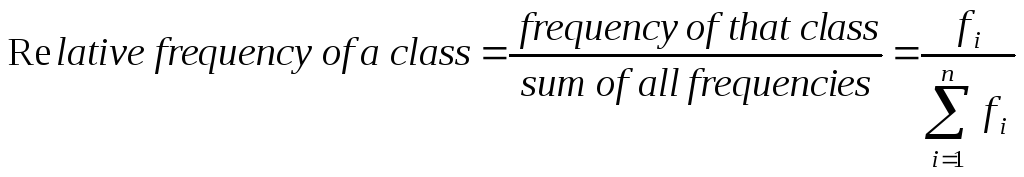
Relative frequency is the proportion of observations in each class. It is defined as:

In addition, we often want to consider the proportion of observations that are either in that or one of the earlier classes. These proportions are called cumulative relative frequencies.

Example in the table 1.9 illustartes how to construct relative frequency and cumulative relative frequency distributions.

Table 1.9

Monthly earnings (in dollars)	Number of employees	Cumulative frequencies	Relative frequencies	Cumulative relative frequencies
301 but less than 400 401 but less than 500 501 but less than 600 601 but less than 700 701 but less than 800 800 but less than 900	4 8 16 10 7 5	4 12 28 38 45 50	4/50 8/50 16/50 10/50 7/50 5/50	4/50=0.08 12/50=0.24 28/50=0.56 38/50=0.76 45/50=0.9 50/50=1
	50		50/50=1	50/50=1

D

efinition:

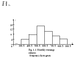
A histogram is a graph in which classes are marked on a horizontal axis and either the frequencies, relative frequencies, or cumulative relative frequencies are marked on the vertical axis. The frequencies, relative frequencies, or cumulative relative frequencies are represented by the heights of the bars. In a histogram, the bars are drawn adjacent

to each other.

Remark:

The symbol “ -//- “ used in the horizontal axis represents a break, called the truncation, in the horizontal axis. It indicates that entire horizontal axis is not shown in this figure. As can be noticed, the zero to 300.5 portion of the horizontal axis has been omitted in the figure 1.1.

As shown in the figure 1.2., we see, for example, that 16/50 of all employees monthly earnings are between 500.5 and 600.5.

T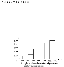he cumulative relative frequencies are the cumulated sums of the relative frequencies. For the first class, the cumulative relative frequency is the same as the relative frequency. For subsequent classes, the cumulative relative frequency for the class to the cumulative relative frequency is obtained by adding the relative frequency for the class to the cumulative relative frequency of the previous class.

The interpretation of these quantities is very valuable. For example, 38/50 of all employees’ monthly earnings are less than 700.5. The information contained in the cumulative relative frequency can also be presented pictorially, as in Fig. 1.3