Young - Computational chemistry

19.6 TRAJECTORY CALCULATIONS

167

corrects for the statistical e¨ects of molecules being drawn out of the ensemble and molecules going back to reactants. This is referred to as calculating the one-way equilibrium ¯ux in the product direction. This results in VTST taking both energy and entropy into account, whereas TST is based on energy only.

Several VTST techniques exist. Canonical variational theory (CVT), improved canonical variational theory (ICVT), and microcanonical variational theory (mVT) are the most frequently used. The microcanonical theory tends to be the most accurate, and canonical theory the least accurate. All these techniques tend to lose accuracy at higher temperatures. At higher temperatures, excited states, which are more di½cult to compute accurately, play an increasingly important role, as do trajectories far from the transition structure. For very small molecules, errors at room temperature are often less than 10%. At high temperatures, computed reaction rates could be in error by an order of magnitude.

For reactions between atoms, the computation needs to model only the translational energy of impact. For molecular reactions, there are internal energies to be included in the calculation. These internal energies are vibrational and rotational motions, which have quantized energy levels. Even with these corrections included, rate constant calculations tend to lose accuracy as the complexity of the molecular system and reaction mechanism increases.

These calculations can also take into account tunneling through the reaction barrier. This is most signi®cant when very light atoms are involved (i.e., hydrogen transfer). Tunneling e¨ects are often included via an approximation method called a semiclassical tunneling calculation. This is an e¨ective onedimensional description of tunneling. This approximation results in the calculation requiring less CPU time without introducing a signi®cant amount of error compared to other ways of including tunneling.

The calculation must be given a description of the potential energy surface either as an analytic function or as the output from molecular orbital calculations. Analytic functions are generally used in order to compare the results of trajectory calculations and VTST calculations for the same surface. Information from molecular calculations might be either a potential energy surface scan or a series of points along the reaction coordinate with their associated gradient and Hessian matrices. Information about the reactants, products, and transition structure, such as geometries and vibrational and rotational excited states, must also be provided. Electronic excited-state information may be necessary if the reaction involves a state crossing. These energy surfaces must be very accurate, often requiring correlated methods with polarized basis sets.

19.6TRAJECTORY CALCULATIONS

Molecular dynamics studies can be done to examine how the path and orientation of approaching reactants lead to a chemical reaction. These studies require an accurate potential energy surface, which is most often an analytic

168 19 REACTION RATES

function ®tted to results from ab initio calculations. Accurate potential energy surfaces have also been obtained from femtosecond spectroscopy results. The amount of work necessary to study a reaction with these techniques may be far more than the work required to obtain the potential energy surface, which was not a trivial task in itself.

A classical trajectory calculation will use this potential energy function in order to run a molecular dynamics simulation. The cross section for reaction can be computed by solving the equations of motion. The rate constants can then be obtained from many trajectories weighted by the appropriate distribution function. Classical trajectory calculations are most accurate for reactions involving heavy atoms at high temperatures. These calculations are sensitive to a number of technical details, such as the choice of the dynamics time step and the choice of numerical integration schemes (see the Karplus, Porter, and Sharma article in the bibliography). Technical details a¨ecting molecular dynamics results are discussed further in Chapter 7.

Quasiclassical calculations are similar to classical trajectory calculations with the addition of terms to account for quantum e¨ects. The inclusion of tunneling and quantized energy levels improves the accuracy of results for light atoms, such as hydrogen transfer, and lower-temperature reactions.

Ab initio trajectory calculations have now been performed. However, these calculations require such an enormous amount of computer time that they have only been done on the simplest systems. At the present time, these calculations are too expensive to be used for computing rate constants, which require many trajectories to be computed. Semiempirical methods have been designed speci®cally for dynamics calculations, which have given insight into vibrational motion, but they have not been the methods of choice for computing rate constants since they are generally inferior to analytic potential energy surfaces ®tted from ab initio results.

19.7STATISTICAL CALCULATIONS

Rather than using transition state theory or trajectory calculations, it is possible to use a statistical description of reactions to compute the rate constant. There are a number of techniques that can be considered variants of the statistical adiabatic channel model (SACM). This is, in essence, the examination of many possible reaction paths, none of which would necessarily be seen in a trajectory calculation. By examining paths that are easier to determine than the trajectory path and giving them statistical weights, the whole potential energy surface is accounted for and the rate constant can be computed.

This technique has not been used as widely as transition state theory or trajectory calculations. The accuracy of results is generally similar to that given by mTST. There are a few cases where SACM may be better, such as for the reactions of some polyatomic polar molecules.

19.9 RECOMMENDATIONS 169

19.8ELECTRONIC STATE CROSSINGS

A simple method for predicting electronic state crossing transitions is Fermi's golden rule. It is based on the electromagnetic interaction between states and is derived from perturbation theory. Fermi's golden rule states that the reaction rate can be computed from the ®rst-order transition matrix H…1† and the density of states at the transition frequency r as follows:

r ˆ	2p	jH…1†j2r	…19:6†
	p

The golden rule is a reasonable prediction of state-crossing transition rates when those rates are slow. Crossings with fast rates are predicted poorly due to the breakdown of the perturbation theory assumption of a small interaction.

There are reaction rates that depend on radiationless transitions between electronic states. For example, photochemically induced reactions often consist of an initial excitation to an excited electronic state, followed by a geometric rearrangement to lower the energy. In the course of this geometric rearrangement, there may be one or more radiationless transitions from one electronic state to another. The rate for these transitions can be obtained from a transition dipole moment calculation, analogous to the transition dipole calculations that give electronic spectrum intensities. For some reactions, spin-orbit coupling is a signi®cant factor in determining the state crossing. A more empirical approach is to use an adiabatic coupling term. It is still a matter of debate which of these techniques is most accurate or most conceptually correct.

19.9RECOMMENDATIONS

Computing reaction rates is not as simple as choosing one more option in an electronic structure program. Deciding to compute reaction rates will require a signi®cant investment of the researchers time in order to understand the various input options. These calculations can give good results, but are very sensitive to subtle details like using a mass-scaled (isoinertial) coordinate system to specify the geometry. Most ab initio programs use center-of-mass or center-of-nuclear- charge coordinates. The computational requirements for completing a reactionrate calculation are fairly modest. The typical calculation will require less than 20 MB of memory and only minutes of CPU time. The POLYRATE software program is the most widely used for performing variational transition state calculations.

For relative reaction rates, ab initio calculations with moderate-size basis sets usually give su½cient accuracy.

For the accurate, a priori calculation of reaction rates, variational transition state calculations are now the method of choice. These calculations are capable of giving the highest-accuracy results, but can be technically di½cult to perform

170 19 REACTION RATES

correctly. They can be done for moderate-size organic molecules. Even with the best of these methods, relative rates are more accurate than absolute rate constants. Absolute rate constants can be in error by as much as a factor of 10 even when the barrier height has been computed to within 1 kcal/mol.

Transition state theory calculations present slightly fewer technical di½culties. However, the accuracy of these calculations varies with the type of reaction. With the addition of an empirically determined correction factor, these calculations can be the most readily obtained for a given class of reactions.

Quasiclassical trajectory calculations are the method of choice for determining the dynamics of intramolecular vibrational energy redistribution leading to a chemical reaction. If this information is desired, an accurate reaction rate can be obtained at little extra expense.

BIBLIOGRAPHY

Introductory descriptions are in

F.Jensen, Introduction to Computational Chemistry John Wiley & Sons, New York (1999).

I. N. Levine, Physical Chemistry Fourth Edition McGraw Hill (1995).

W. H. Green, Jr., C. B. Moore, W. P. Polik, Ann. Rev. Phys. Chem. 43, 591 (1992).

D. M. Hirst, A Computational Approach to Chemistry Blackwell Scienti®c, Oxford (1990).

R. Daudel, Adv. Quantum Chem. 3, 161 (1967).

D. G. Truhlar, B. C. Garret, Acc. Chem. Res. 13, 440 (1980).

Introductory descriptions of trajectory calculations are

D. L. Bunker, Methods Comput. Phys. 10, 287 (1971).

M. Karplus, R. N. Porter, R. D. Sharma, J. Chem. Phys. 43, 3259 (1965).

Relative reaction rate comparisons are discussed in

W. J. Hehre, Practical Strategies for Electronic Structure Calculations Wavfunction, Irvine (1995).

The most hands on description of doing these calculations is in the software manuals, such as

R. Steckler, Y.-Y. Chuang, E. L. Coitino, W.-P. Hu, Y.-P. Lin, G. C. Lynch, K. A. Nguyen, C. F. Jackels, M. Z. Gu, I. Rossi, P. Fast, S. Clayton, V. S. Melissas, B. C. Garrett, A. D. Isaacson, D. G. Truhlar, POLYRATE Manual (1999).

Mathematical developments of reaction rate theory are given in

G. C. Schatz, M. A. Ratner, Quantum Mechanics in Chemistry Prentice Hall (1993). D. G. Truhlar, A. D. Isaacson, B. C. Garrett, Theory of Chemical Reaction Dynamics

Vol. IV M. Baer Ed., 65, CRC (1985).

BIBLIOGRAPHY 171

A review of reactions in solution is

J.T. Hynes, Theory of Chemical Reaction Dynamics Volume IV B. Bauer, Ed., 171, CRC, Boca Raton (1985).

Reviews of transition state theory and variational transition state theory are

W. H. Miller, Encycl. Comput. Chem. 4, 2375 (1998).

M. Quack, J. Troe, Encycl. Comput. Chem. 4, 2708 (1998).

B. C. Garrett, D. G. Truhlar, Encycl. Comput. Chem. 5, 3094 (1998).

D. G. Truhlar, B. C. Garrett, S. J. Klippenstein, J. Phys. Chem. 100, 12771 (1996).

A.D. Isaacson, D. G. Truhlar, S. N. Rai, R. Steckler, G. C. Hancock, B. C. Garrett, M. J. Redmon, Comp. Phys. Commun. 47, 91 (1987).

M.M. Kreevoy, D. G. Truhlar, Investigation of Rates and Mechanisms of Reactions, Part 1, 4th Edition C. F. Bernasconi Ed., 13, John Wiley, New York (1986).

T.Fonseca, J. A. N. F. Gomes, P. Grigolini, F. Marchesoni, Adv. Chem. Phys. 62, 389 (1985).

K.J. Laidler, M. C. King, J. Phys. Chem. 87, 2657 (1983).

D.G. Truhlar, W. L. Hase, J. T. Hynes, J. Phys. Chem. 87, 2664 (1983).

P.Pechukas, Ann. Rev. Phys. Chem. 32, 159 (1981).

R.B. Walker, J. C. Light, Ann. Rev. Phys. Chem. 31, 401 (1980).

T.F. George, J. Ross, Ann. Rev. Phys. Chem. 24, 263 (1973).

J.C. Light, Adv. Chem. Phys. 19, 1 (1971).

E.V. Waage, B. S. Rabinovitch, Chem. Rev. 70, 377 (1970).

J. C. Keck, Adv. Chem. Phys. 13, 85 (1967).

Reviews of trajectory calculations are

G. D. Billing, Encycl. Comput. Chem. 3, 1587 (1998).

G. D. Billing, K. V. Mikkelsen, Introduction to Molecular Dynamics and Chemical Kinetics John Wiley & Sons, New York (1996).

J. M. Bowman, G. C. Schatz, Ann. Rev. Phys. Chem. 46, 169 (1995).

Bimolecular Collisions M. N. R. Ashford, J. E. Battott, Eds., Royal Society of Chemistry, Herts (1989).

G. C. Schatz, Ann. Rev. Phys. Chem. 39, 317 (1988). D. G. Truhlar, J. Phys. Chem. 83, 188 (1979).

D.G. Truhlar, J. T. Muckerman, Atom-Molecule Collision Theory. A Guide for the Experimentalist R. B. Bernstein, Ed., 505, Plenum (1979).

R. N. Porter, Ann. Rev. Phys. Chem. 25, 317 (1974).

B.Widom, Adv. Chem. Phys. 5, 353 (1963).

Tunneling in reactions is reviewed in

E. F. Caldin, Chem. Rev. 69, 135 (1969).

H. S. Johnston, Adv. Chem. Phys. 3, 131 (1961).

172 19 REACTION RATES

Radiationless transition calculations are described in

M. Klessinger, Theoretical Organic Chemistry C. PaÂrkaÂni Ed., 581, Elsevier (1998).

J. Simons, J. Nichols, Quantum Mechanics in Chemistry 314, Oxford, New York (1997). V. V. Kocharovsky, V. V. Kocharovsky, S. Tasaki, Adv. Chem. Phys. 99, 333 (1997). Adv. Chem. Phys. P. Gaspard, I. Burghardt, Eds., 101 (1997).

R. H. Landau, Quantum Mechanics II; A Second Course in Quantum Theory Second Edition 314, John Wiley & Sons, New York (1996).

F. Bernardi, M. Olivucci, M. A. Robb, Chem. Soc. Rev. 25, 321 (1996).

L.Serrano-Andres, M. Merchan, I. Nebot-Gil, R. Lindh, B. O. Roos, J. Chem. Phys. 98, 3151 (1993).

Adv. Chem. Phys. M. Baer, C. ±Y. Ng, Eds., 82 (1992).

M. Baer, Theory of Chemical Reaction Dynamics Vol. II M. Baer Ed., 219, CRC (1985). A. A. Ovchinnikov, M. Y. Ovchinnokova, Adv. Quantum Chem. 16, 161 (1982).

C.Cohen-Tannoudji, B. Diu, F. LaloeÈ, Quantum Mechanics 1299, John Wiley & Sons, New York (1977).

E.E. Nikitin, Adv. Quantum Chem. 5, 135 (1970).

Statistical calculations are reviewed in

J. Troe, Adv. Chem. Phys. 101, 819 (1997).

D. A. McQuarrie, Adv. Chem. Phys. 15, 149 (1969).

Computational Chemistry: A Practical Guide for Applying Techniques to Real-World Problems. David C. Young Copyright ( 2001 John Wiley & Sons, Inc.

ISBNs: 0-471-33368-9 (Hardback); 0-471-22065-5 (Electronic)

20 Potential Energy Surfaces

In the chapter on reaction rates, it was pointed out that the perfect description of a reaction would be a statistical average of all possible paths rather than just the minimum energy path. Furthermore, femtosecond spectroscopy experiments show that molecules vibrate in many di¨erent directions until an energetically accessible reaction path is found. In order to examine these ideas computationally, the entire potential energy surface (PES) or an approximation to it must be computed. A PES is either a table of data or an analytic function, which gives the energy for any location of the nuclei comprising a chemical system.

20.1PROPERTIES OF POTENTIAL ENERGY SURFACES

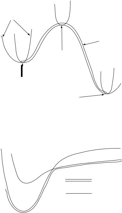
Once a PES has been computed, it can be analyzed to determine quite a bit of information about the chemical system. The PES is the most complete description of all the conformers, isomers, and energetically accessible motions of a system. Minima on this surface correspond to optimized geometries. The lowest-energy minimum is called the global minimum. There can be many local minima, such as higher-energy conformers or isomers. The transition structure between the reactants and products of a reaction is a saddle point on this surface. A PES can be used to ®nd both saddle points and reaction coordinates. Figure 20.1 illustrates these topological features. One of the most common reasons for doing a PES computation is to subsequently study reaction dynamics as described in Chapter 19. The vibrational properties of the molecule can also be obtained from the PES.

In describing PES, the terms adiabatic and diabatic are used. In the older literature, these terms are used in confusing and sometimes con¯icting ways. For the purposes of this discussion, we will follow the conventions described by Sidis; they are both succinct and re¯ective of the most common usage. The term adiabatic originated in thermodynamics, where it means no heat transfer …dq ˆ 0†. An adiabatic PES is one in which a particular electronic state is followed; thus no transfer of electrons between electronic states occurs. Only in a few rare cases is this distinction noted by using the term electronically adiabatic. A diabatic surface is the lowest-energy state available for each set of nuclear positions, regardless of whether it is necessary to switch from one electronic state to another. These are illustrated in Figure 20.2.

173

174 20 POTENTIAL ENERGY SURFACES

PES

IRC path

saddle point

local minimum

global minimum

FIGURE 20.1 Points on a potential energy surface.

The mathematical de®nition of the Born±Oppenheimer approximation implies following adiabatic surfaces. However, software algorithms using this approximation do not necessarily do so. The approximation does not re¯ect physical reality when the molecule undergoes nonradiative transitions or two

adiabatic paths

diabatic path

FIGURE 20.2 Adiabatic paths for bond dissociation in two di¨erent electronic states and the diabatic path.

20.2 COMPUTING POTENTIAL ENERGY SURFACES 175

electronic states are intimately involved in a process, such as Jahn±Teller distortions or vibronic coupling e¨ects.

Depending on the information desired, the researcher might wish to have a calculation follow either an adiabatic path or a diabatic path, as shown in Figure 20.2. Which potential energy surface is followed depends on both the construction of the wave function and the means by which wave function symmetry is used by the software. A single-determinant wave function in which wave function symmetry is imposed will follow the adiabatic surface where two states of di¨erent symmetry cross. When two states of the same symmetry cross, a single-determinant wave function will exhibit an avoided crossing, as shown in Figure 17.2. A multiple-determinant wave function, in which both states are in the con®guration space, will have the ¯exibility to follow the diabatic path. It is sometimes possible to get a multiple-determinant calculation (particularly MCSCF) to follow the adiabatic path by moving in small steps and using the optimized wave function from the previous point as the initial guess for each successive step.

20.2COMPUTING POTENTIAL ENERGY SURFACES

Computing a complete PES for a molecule with N atoms requires computing energies for geometries on a grid of points in 3N-6 dimensional space. This is extremely CPU-intensive because it requires computing a set of X points in each dimension, resulting in X 3N-6 single point computations. Because of this, PES's are typically only computed for systems with a fairly small number of atoms.

Some software packages have an automated procedure for computing all the points on a PES, but a number of technical problems commonly arise. Some programs have a function that halts the execution when two nuclei are too close together; this function must be disabled. SCF procedures often exhibit convergence problems far from equilibrium. Methods for ®xing SCF convergence problems are discussed in Chapter 22. At di¨erent points on the PES, the molecule may have di¨erent symmetries. This often results in errors when using software packages that use molecular symmetry to reduce computation time. The use of symmetry by a program can often be turned o¨. Computation of the PES for electronic excited states can lead to additional technical di½culties as described in Chapter 25.

The level of theory necessary for computing PES's depends on how those results are to be used. Molecular mechanics calculations are often used for examining possible conformers of a molecule. Semiempiricial calculations can give a qualitative picture of a reaction surface. Ab initio methods must often be used for quantitatively correct reaction surfaces. Note that size consistent methods must be used for the most accurate results. The speci®c recommendations given in Chapter 18 are equally applicable to PES calculations.

176 20 POTENTIAL ENERGY SURFACES

20.3FITTING PES RESULTS TO ANALYTIC EQUATIONS

Once a PES has been computed, it is often ®tted to an analytic function. This is done because there are many ways to analyze analytic functions that require much less computation time than working directly with ab initio calculations. For example, the reaction can be modeled as a molecular dynamics simulation showing the vibrational motion and reaction trajectories as described in Chapter 19. Another technique is to ®t ab initio results to a semiempirical model designed for the purpose of describing PES's.

Of course, the analytic surface must be fairly close to the shape of the true potential in order to obtain physically relevant results. The criteria on ®tting PES results to analytic equations have been broken down into a list of 10 speci®c items, all of which have been discussed by a number of authors. Below is the list as given by Schatz:

1.The analytic function should accurately characterize the asymptotic reactant and product molecules.

2.It should have the correct symmetry properties of the system.

3.It should represent the true potential accurately in the interaction regions for which experimental or nonempirical theoretical data are available.

4.It should behave in a physically reasonable manner in those parts of the interaction regions for which no experimental or theoretical data are available.

5.It should smoothly connect the asymptotic and interaction regions in a physically reasonable way.

6.The interpolating function and its derivatives should have as simple an algebraic form as possible consistent with the desired goodness of ®t.

7.It should require as small a number of data points as possible to achieve an accurate ®t.

8.It should converge to the true surface as more data become available.

9.It should indicate where it is most meaningful to compute the data points.

10.It should have a minimal amount of ``ad hoc'' or ``patched up'' character.

Criteria 1 through 5 must be obeyed in order to obtain reasonable results in subsequent calculations using the function. Criteria 6 through 10 are desirable for practical reasons. Finding a function that meets these criteria requires skill and experience, and no small amount of patience.

The analytic PES function is usually a summation of twoand three-body terms. Spline functions have also been used. Three-body terms are often polynomials. Some of the two-body terms used are Morse functions, Rydberg