Young - Computational chemistry

120 13 OTHER CHEMICAL PROPERTIES

FIGURE 13.6 A plot showing two data values. The shape is an isosurface of the total electron density. The color applied to the surface is based on the magnitude of the electrostatic potential at that point in space.

the wave function and use them to create a graphical representation without the intermediate step of storing the data.

Some limitations are purely a matter of the functionality of the program. For example, some programs will not render images with a white background (generally best for publication on white paper) or include a function to save the image in a format that can be used by typical word processing software. Some programs give the user a large amount of control over the rendering settings, whereas others force the user to use a default set of options.

There is often a fundamental disparity between the graphic ability of computer monitors and that of printers. Monitors may use anywhere from 8-bit color (256 colors) to 24-bit color (16 million colors). Printers, except for dye sublimation models, use four colors, which are printed in a pattern that tricks the eye into seeing all colors. Monitors generally use about a 72-dpi (dots per inch) screen resolution, as compared to printer resolutions of 300 dpi or better.

There are also two ways to store and use image data. A raster-drawn (or bitmapped) image is one composed of many evenly spaced dots, each given a particular color. A vector-drawn image is described by lines and curves with various lengths and curvatures. Raster-drawn images are very common because they most readily created by almost any type of software. Files with gif, jpg, jpeg, and bmp extensions are raster-drawn image ®les. The advantage of using

BIBLIOGRAPHY 121

vector-drawn images is that they give the best possible line quality on both the computer monitor and printer. The ChemDraw program uses vector-drawn images. Postscript supports both raster and vector formats.

13.16CONCLUSIONS

Completely ab initio predictions can be more accurate than any experimental result currently available. This is only true of properties that depend on the behavior of isolated molecules. Colligative properties, which are due to the interaction between molecules, can be computed more reliably with methods based on thermodynamics, statistical mechanics, structure-activity relationships, or completely empirical group additivity methods.

Empirical methods, such as group additivity, cannot be expected to be any more accurate than the uncertainty in the experimental data used to parameterize them. They can be much less accurate if the functional form is poorly chosen or if predicting properties for compounds signi®cantly di¨erent from those in the training set.

Researchers must be particularly cautious when using one estimated property as the input for another estimation technique. This is because possible error can increase signi®cantly when two approximate techniques are combined. Unfortunately, there are some cases in which this is the only available method for computing a property. In this case, researchers are advised to work out the error propagation to determine an estimated error in the ®nal answer.

An example of using one predicted property to predict another is predicting the adsorption of chemicals in soil. This is usually done by ®rst predicting an octanol water partition coe½cient and then using an equation that relates this to soil adsorption. This type of property±property relationship is most reliable for monofunctional compounds. Structure±property relationships, and to a lesser extent group additivity methods, are more reliable for multifunctional compounds than this type of relationship.

BIBLIOGRAPHY

Books pertinent to this chapter are

E.J. Baum, Chemical Property Estimation: Theory and Applications Lewis, Boca Raton (1998).

A. R. Leach, Molecular Modelling Principles and Applications Longman, Essex (1996).

G.A. Je¨rey, J. F. Piniela, The Application of Charge Density Research to Chemistry and Drug Design Plenum, New York (1991).

W.J. Lyman, W. F. Reehl, D. H. Rosenblatt, Handbook of Chemical Property Estimation Methods American Chemical Society, Washington (1990).

122 13 OTHER CHEMICAL PROPERTIES

C. E. Dykstra, Ab Initio Calculation of the Structures and Properties of Molecules

Elsevier, Amsterdam (1988).

R.C. Reid, J. M. Prausnitz, The Properties of Gases and Liquids McGraw Hill, New York (1987).

M. P. Allen, D. J. Tildesley, Computer Simulation of Liquids Oxford, Oxford (1987).

Chemical Applications of Atomic and Molecular Electrostatic Potentials P. Politzer, D. G. Truhlar, Eds., Plenum, New York (1981).

G. J. Janz, Thermodynamic Properties of Organic Compounds Academic Press, New York (1967).

Reviews of using arti®cial intelligence to predict properties are

J.Zupan, J. Gasteiger, Neural Networks in Chemistry and Drug Design John Wiley & Sons, New York (1999).

D. H. Rouvray, Fuzzy Logic in Chemistry Academic Press, San Diego (1997).

F. J. Smith, M. Sullivan, J. Collis, S. Loughlin, Adv. Quantum Chem. 28, 319 (1997). W. Duch, Adv. Quantum Chem. 28, 329 (1997).

P. L. Kilpatrick, N. S. Scott, Adv. Quantum Chem. 28, 345 (1997).

H. M. Cartwright, Applications of Arti®cial Intelligence in Chemistry Oxford, Oxford (1993).

Reviews of dielectric constant prediction are

S. W. de Leeuw, J. W. Perrom, E. R. Smith, Ann. Rev. Phys. Chem. 37, 245 (1986).

B.J. Alder, E. L. Pollock, Ann. Rev. Phys. Chem. 32, 311 (1981).

A review of electron a½nity and ionization potential prediction are

J.S. Murray, P. Politzer, Theoretical Organic Chemistry C. PaÂrkaÂnyi, Ed., 189, Elsevier, Amsterdam (1998).

G.L. Gutsev, A. I. Boldyrev, Adv. Chem. Phys. 61, 169 (1985).

A review of electrostatic potential analysis is

T.Brinck, Theoretical Organic Chemistry C. PaÂrkaÂnyi, Ed., 51, Elsevier, Amsterdam (1998).

P. Politzer, J. S. Murray, Rev. Comput. Chem. 2, 273 (1991).

E. Scrocco, J. Tomasi, Adv. Quantum Chem. 11, 116 (1978).

Hardness and electronegativity are addressed in

R. G. Pearson, Theoretical Models of Chemical Bonding Part 2 Z. B. MaksicÂ, Ed., Springer-Verlag, Berlin (1990).

Reviews of hyper®ne coupling prediction are

L. A. Eriksson, Encycl. Comput. Chem. 2, 952 (1998).

S. M. Blinder, Adv. Quantum Chem. 2, 47 (1965).

BIBLIOGRAPHY 123

Reviews of multipole computation are

C.PaÂrkaÂnyi, J.-J. Aaron, Theoretical Organic Chemistry C. PaÂrkaÂnyi, Ed., 233, Elsevier, Amsterdam (1998).

I. B. Bersuker, I. Y. Ogurtsov, Adv. Quantum Chem. 18, 1 (1986).

S. Green, Adv. Chem. Phys. 25, 179 (1974).

Articles addressing optical activity computation are

A. Rauk, Encycl. Comput. Chem. 1, 373 (1998).

R. K. Kondru, P. Wipf, D. N. Beratan, Science 282, 2247 (1998).

D. Yang, A. Rouk, Rev. Comput. Chem. 7, 261 (1996).

F. S. Richardson, Chem. Rev. 79, 17 (1979).

A. Moscowitz, Adv. Chem. Phys. 4, 67 (1962).

I. Tinoco, Jr., Adv. Chem. Phys. 4, 113 (1962).

Reviews of molecular similarity are

R. CarboÂ, B. Calabuig, L. Vera, E. BesaluÂ, Adv. Quantum Chem. 25, 253 (1994).

Reviews of molecular size and volume are

M. L. Connolly, Encycl. Comput. Chem. 3, 1698 (1998).

A. Y. Meyer, Chem. Soc. Rev. 15, 449 (1986).

A review of chemical toxicity prediction is

D. F. V. Lewis, Rev. Comput. Chem. 3, 173 (1992).

A review of Walsh diagram prediction is

R. J. Buenker, S. D. Peyerimho¨, Chem. Rev. 74, 127 (1974).

Reviews of visualization techniques are

T. E. Ferrin, T. E. Klein, Encycl. Comput. Chem. 1, 463 (1998).

J. Brickmann, T. Exner, M. Keil, R. MarhoÈfer, G. Moeckel, Encycl. Comput. Chem. 3, 1678 (1998).

P. G. Mezey, Encycl. Comput. Chem. 4, 2582 (1998).

Chemical Hardness K. D. Sen, Ed., Springer-Verlag, Berlin (1993). P. G. Mezey, Rev. Comput. Chem. 1, 265 (1990).

S. Andersson, S. T. Hyde, K. Larsson, S. Lidin, Chem. Rev. 88, 221 (1988). Electronegativity K. D. Sen, C. K. Jorgensen, Eds., Springer-Verlag, Berlin (1987).

A. Hinchli¨, Ab Initio Determination of Molecular Properties Adam Hilger, Bristol (1987).

R.F. Hout, Jr., W. J. Pietro, W. J. Hehre, A Pictorial Approach to Molecular Structure and Reactivity John Wiley & Sons, New York (1984).

P. Coppens, E. D. Steven, Adv. Quantum Chem. 10, 1 (1977).

124 13 OTHER CHEMICAL PROPERTIES

A. Hinchli¨e, J. C. Dobson, Chem. Soc. Rev. 5, 79 (1976).

W. L. Jorgensen, The Organic Chemists Book of Orbitals Academic Press, New York (1973).

A review of visualizing reaction coordinates is

O. M. Becker, J. Comput. Chem. 19, 1255 (1998).

Other relevant reviews are

C. E. Dykstra, S.-Y. Liu, D. J. Malik, Adv. Chem. Phys. 75, 37 (1989). L. Engelbrecht, J. Hinze, Adv. Chem. Phys. 44, 1 (1980).

J.R. Van Wazer, I. Absar, Electron Densities in Molecules and Molecular Orbitals

Academic Press, New York (1975).

G. G. Hall, Adv. Quantum Chem. 1, 241 (1964).

Computational Chemistry: A Practical Guide for Applying Techniques to Real-World Problems. David C. Young Copyright ( 2001 John Wiley & Sons, Inc.

ISBNs: 0-471-33368-9 (Hardback); 0-471-22065-5 (Electronic)

14 The Importance of Symmetry

This chapter discusses the application of symmetry to orbital-based computational chemistry problems. A number of textbooks on symmetry are listed in the bibliography at the end of this chapter.

The symmetry of a molecule is de®ned by determining how the nuclei can be exchanged without changing its identity, conformation, or chirality. For example, a methane molecule can be turned about the axis connecting the carbon and one of the hydrogens by 120 and it is indistinguishable from the original orientation. Alternatively, symmetry can be considered a way of determining which regions of space around the molecule are completely equivalent. This second description is important because it indicates a means for calculations to be performed more quickly.

In order to obtain this savings in the computational cost, orbitals are symmetry-adapted. As various positive and negative combinations of orbitals are used, there are a number of ways to break down the total wave function. These various orbital functions will obey di¨erent sets of symmetry constraints, such as having positive or negative values across a mirror plane of the molecule. These various symmetry sets are called irreducible representations.

Molecular orbitals are not unique. The same exact wave function could be expressed an in®nite number of ways with di¨erent, but equivalent orbitals. Two commonly used sets of orbitals are localized orbitals and symmetryadapted orbitals (also called canonical orbitals). Localized orbitals are sometimes used because they look very much like a chemist's qualitative models of molecular bonds, lone-pair electrons, core electrons, and the like. Symmetryadapted orbitals are more commonly used because they allow the calculation to be executed much more quickly for high-symmetry molecules. Localized orbitals can give the fastest calculations for very large molecules without symmetry due to many long-distance interactions becoming negligible.

Another reason that symmetry helps the calculations is that the Hamiltonian matrix will become a block diagonal matrix with one block for each irreducible representation. It is not necessary for the program to compute overlap integrals between orbitals of di¨erent irreducible representations since the overlap integrals will be zero by symmetry. Some computer programs go to the length of actually completing an SCF calculation as a number of small Hamiltonian matrices for each irreducible representation rather than one large Hamiltonian matrix. When this is done, the number of orbitals of each irreducible representation that are occupied must be de®ned at the beginning of the calculation

125

126 14 THE IMPORTANCE OF SYMMETRY

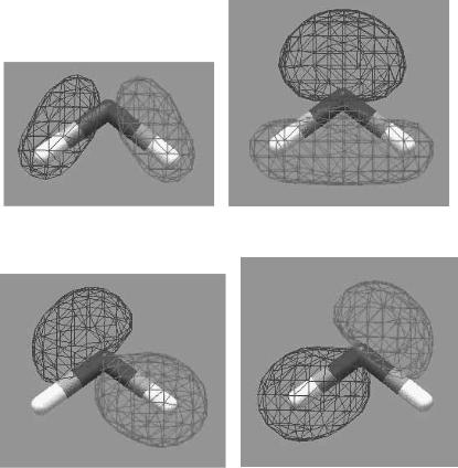
(a) B2 orbital

(b) A1 orbital

(c) B2 + A1	(d) B2 - A1

FIGURE 14.1 An illustration of symmetry-adapted vs. localized orbitals for water. (a, b) B2 and A1 symmetry-adapted orbitals. (c) Sum of these orbitals, which gives a localized orbital that is the bond between the oxygen and the hydrogen on the right. (d ) Di¨erence between these orbitals, which gives a localized orbital that is the bond between the oxygen and the hydrogen on the left.

either by the user or the program. Electrons will not be able to shift from one symmetry to another. Thus, the ground-state wave function cannot be determined unless the correct electron symmetry assignments were chosen originally. This can be an advantage since it is a way of obtaining excited-state wave functions, and fewer SCF convergence problems arise with this algorithm. The disadvantage is that the automated assignment algorithm may not ®nd the correct ground state.

There is always a transformation between symmetry-adapted and localized orbitals that can be quite complex. A simple example would be for the bonding orbitals of the water molecule. As shown in Figure 14.1, localized orbitals can

BIBLIOGRAPHY 127

be constructed from positive and negative combinations of symmetry-adapted orbitals. Some computer programs have localization algorithms that are more sophisticated than this.

14.1WAVE FUNCTION SYMMETRY

In SCF problems, there are some cases where the wave function must have a lower symmetry than the molecule. This is due to the way that the wave function is constructed from orbitals and basis functions. For example, the carbon monoxide molecule might be computed with a wave function of C4v symmetry even though the molecule has a Cyv symmetry. This is because the orbitals obey C4v constraints.

Most programs that employ symmetry-adapted orbitals only use Abelian symmetry groups. Abelian groups are point groups in which all the symmetry operators commute. Often, the program will ®rst determine the molecules' symmetry and then use the largest Abelian subgroup. To our knowledge, the only software package that can utilize non-Abelian symmetry groups is Jaguar.

14.2TRANSITION STRUCTURES

Transition structures can be de®ned by nuclear symmetry. For example, a symmetric SN 2 reaction will have a transition structure that has a higher symmetry than that of the reactants or products. Furthermore, the transition structure is the lowest-energy structure that obeys the constraints of higher symmetry. Thus, the transition structure can be calculated by forcing the molecule to have a particular symmetry and using a geometry optimization technique.

BIBLIOGRAPHY

T. Bally, W. T. Borden, Rev. Comput. Chem. 13, 1 (1999).

J. Rosen, Symmetry in Science Springer-Verlag, New York (1996).

G.Davidson, Group Theory for Chemists MacMillan, Hampshire (1991).

A.Cotton, Chemical Applications of Group Theory John Wiley and Sons, New York (1990).

J.R. Ferraro, J. S. Ziomek, Introductory Group Theory Plenum, New York (1975).

D. M. Bishop, Group Theory and Chemistry Clarendon, Oxford (1973).

M. Tinkham, Group Theory and Quantum Mechanics McGraw-Hill, New York (1964). R. McWeeny, Symmetry; An Introduction to Group Theory and its Applications

Pergamon, New York (1963).

Computational Chemistry: A Practical Guide for Applying Techniques to Real-World Problems. David C. Young Copyright ( 2001 John Wiley & Sons, Inc.

ISBNs: 0-471-33368-9 (Hardback); 0-471-22065-5 (Electronic)

E½cient Use of Computer

15 Resources

Many computational chemistry techniques are extremely computer-intensive. Depending on the type of calculation desired, it could take anywhere from seconds to weeks to do a single calculation. There are many calculations, such as ab initio analysis of biomolecules, that cannot be done on the largest computers in existence. Likewise, calculations can take very large amounts of computer memory and hard disk space. In order to complete work in a reasonable amount of time, it is necessary to understand what factors contribute to the computer resource requirements. Ideally, the user should be able to predict in advance how much computing power will be needed.

There are often trade-o¨s between equivalent ways of doing the same calculation. For example, many ab initio programs use hard disk space to store numbers that are computed once and used several times during the course of the calculation. These are the integrals that describe the overlap between various basis functions. Instead of the above method, called conventional integral evaluation, it is possible to use direct integral evaluation in which the numbers are recomputed as needed. Direct integral evaluation algorithms use less disk space at the expense of requiring more CPU time to do the calculation. An incore algorithm is one that stores all the integrals in RAM memory, thus saving on disk space at the expense of requiring a computer with a very large amount of memory. Many programs use a semidirect algorithm, which uses some disk space and a bit more CPU time to obtain the optimal balance of both.

15.1TIME COMPLEXITY

Time complexity is a way of denoting how the use of computer resources (CPU time, memory, etc.) changes as the size of the problem changes. For example, consider a HF calculation with N orbitals. At the end of the calculation, the orbital energies must be added. Since there are N orbitals, there will be N addition operations. There are a certain number of operations, which we will call C, which have to be done regardless of the size of calculation, such as initializing variables and allocating memory. The standard matrix inversion algorithm requires N 3 operations. Computing the two-electron Coulomb and exchange integrals for a HF calculation takes N 4 operations. Thus, the total amount of CPU time required to do a HF calculation scales as N 4 ‡ N 3 ‡ N ‡ C. However for su½ciently large N, the N 3, N, and C terms are insigni®cant compared

128

						15.1 TIME COMPLEXITY		129
to3the size of	the N 4 term (if N			ˆ	10, then N 3	is 10% of N 4, and for N	ˆ	100,
	N	4
N is 1% of			, etc.). Computer scientists described this type of algorithm as

one that has a time complexity of N 4, denoted with the notation O…N 4†. A similar analysis could be done for memory use, disk use, network communication volume, and so on.

These relationships can be used to estimate the amount of CPU time, disk space, or memory needed to run calculations. Let us take the example of a researcher, Jane Chemist, who would like to compute some property of a polymer. She ®rst examines the literature to determine that an ab initio method with a moderately large basis set will give the desired accuracy of results. She then runs both single point and geometry optimization calculations on the monomer, which take 2 and 20 minutes, respectively. Since the calculation scales as N 4, a geometry optimization for the trimer, which has three times as many atoms, will take approximately 34 20 minutes or about 27 hours. Jane would like to model up to a 15-unit chain, which would require 154 20 minutes or about 2 years. Obviously, the use of ab initio methods for geometry optimization is not acceptable. Jane then wisely decides to stop at the 10-unit chain and use geometries optimized with molecular mechanics methods, which takes under an hour for the optimization. She then obtains the desired results with singlepoint ab initio calculations, which take 104 2 minutes or 2 weeks for the largest molecule. This ®nal calculation is still rather large, but it is feasible since Jane has her own work station with an uninterruptable power supply.

There are many di¨erent algorithms that can be programmed in a more or less e½cient manner to obtain the exact same result. Because of this, a given method will have slightly di¨erent time complexities from one program to another. Table 15.1 gives some common time complexities. M is the number of atoms, L the length of one side of the box containing the molecules in a calculation using periodic boundary conditions, A the number of active space orbitals, and N the number of orbitals in the calculation. Thus, N can increase either by including more atoms or using a larger basis set.

Geometry optimization calculations take much longer than single-energy calculations. The reasons are two-fold: First, many calculations must be done as the geometry is changed. Second, each iteration takes longer in order to compute energy gradients. The amount of CPU time required for a geometry optimization, Topt, depends on the number of degrees of freedom, denoted as D. Degrees of freedom are the geometric variables being optimized, such as bond lengths, angles, and the like. As a general rule of thumb, the amount of time for a geometry optimization can be estimated from the single-point energy CPU time, Tsingle, with the equation

Topt G 5 D2 Tsingle

…15:1†

For ab initio, semiempirical, or molecular dynamics calculations, the amount of CPU time necessary is generally the factor of greatest concern to researchers. For very large molecules, memory use is of concern for molecular mechanics