Young - Computational chemistry

Computational Chemistry: A Practical Guide for Applying Techniques to Real-World Problems. David C. Young Copyright ( 2001 John Wiley & Sons, Inc.

ISBNs: 0-471-33368-9 (Hardback); 0-471-22065-5 (Electronic)

Molecular Dynamics and Monte

7 Carlo Simulations

In Chapter 2, a brief discussion of statistical mechanics was presented. Statistical mechanics provides, in theory, a means for determining physical properties that are associated with not one molecule at one geometry, but rather, a macroscopic sample of the bulk liquid, solid, and so on. This is the net result of the properties of many molecules in many conformations, energy states, and the like. In practice, the di½cult part of this process is not the statistical mechanics, but obtaining all the information about possible energy levels, conformations, and so on. Molecular dynamics (MD) and Monte Carlo (MC) simulations are two methods for obtaining this information

7.1MOLECULAR DYNAMICS

Molecular dynamics is a simulation of the time-dependent behavior of a molecular system, such as vibrational motion or Brownian motion. It requires a way to compute the energy of the system, most often using a molecular mechanics calculation. This energy expression is used to compute the forces on the atoms for any given geometry. The steps in a molecular dynamics simulation of an equilibrium system are as follows:

1.Choose initial positions for the atoms. For a molecule, this is whatever geometry is available, not necessarily an optimized geometry. For liquid simulations, the molecules are often started out on a lattice. For solvent± solute systems, the solute is often placed in the center of a collection of solvent molecules, with positions obtained from a simulation of the neat solvent.

2.Choose an initial set of atom velocities. These are usually chosen to obey a Boltzmann distribution for some temperature, then normalized so that the net momentum for the entire system is zero (it is not a ¯owing system).

3.Compute the momentum of each atom from its velocity and mass.

4.Compute the forces on each atom from the energy expression. This is usually a molecular mechanics force ®eld designed to be used in dynamical simulations.

5.Compute new positions for the atoms a short time later, called the time step. This is a numerical integration of Newton's equations of motion using the information obtained in the previous steps.

60

7.1 MOLECULAR DYNAMICS 61

6.Compute new velocities and accelerations for the atoms.

7.Repeat steps 3 through 6.

8.Repeat this iteration long enough for the system to reach equilibrium. In this case, equilibrium is not the lowest energy con®guration; it is a con- ®guration that is reasonable for the system with the given amount of energy.

9.Once the system has reached equilibrium, begin saving the atomic coordinates every few iterations. This information is typically saved every 5 to 25 iterations. This list of coordinates over time is called a trajectory.

10.Continue iterating and saving data until enough data have been collected to give results with the desired accuracy.

11.Analyze the trajectories to obtain information about the system. This might be determined by computing radial distribution functions, di¨u- sion coe½cients, vibrational motions, or any other property computable from this information.

In order for this to work, the force ®eld must be designed to describe intermolecular forces and vibrations away from equilibrium. If the purpose of the simulation is to search conformation space, a force ®eld designed for geometry optimization is often used. For simulating bulk systems, it is more common to use a force ®eld that has been designed for this purpose, such as the GROMOS or OPLS force ®elds.

There are several algorithms available for performing the numerical integration of the equations of motion. The Verlet algorithm is widely used because it requires a minimum amount of computer memory and CPU time. It uses the positions and accelerations of the atoms at the current time step and positions from the previous step to compute the positions for the next time step. The velocity Verlet algorithm uses positions, velocities, and accelerations at the current time step. This gives a more accurate integration than the Verlet algorithm. The Verlet and velocity Verlet algorithms often have a step in which the velocities are rescaled in order to correct for minor errors in the integration, thus simulating a constant-temperature system. Beeman's algorithm uses positions, velocities, and accelerations from the previous time step. It gives better energy conservation at the expense of computer memory and CPU time. A Gear predictor-corrector algorithm predicts the next set of positions and accelerations, then compares the accelerations to the predicted ones to compute a correction for the step. Each step can thus be re®ned iteratively. Predictorcorrector algorithms give an accurate integration but are seldom used due to their large computational needs.

The choice of a time step is also important. A time step that is too large will cause atoms to move too far along a given trajectory, thus poorly simulating the motion. A time step that is too small will make it necessary to run more iterations, thus taking longer to run the simulation. One general rule of thumb is that the time step should be one order of magnitude less than the timescale of

62 7 MOLECULAR DYNAMICS AND MONTE CARLO SIMULATIONS

the shortest motion (vibrational period or time between collisions). This gives a time step on the order of tens of femtoseconds for simulating a liquid of rigid molecules and tenths of a femtosecond for simulating vibrating molecules.

It is important to verify that the simulation describes the chemical system correctly. Any given property of the system should show a normal (Gaussian) distribution around the average value. If a normal distribution is not obtained, then a systematic error in the calculation is indicated. Comparing computed values to the experimental results will indicate the reasonableness of the force ®eld, number of solvent molecules, and other aspects of the model system.

The algorithm described above is for a system with a constant volume, number of particles, and temperature. It is also possible to set up a calculation in which the velocities are rescaled slightly at each step to simulate a changing temperature. For solvent±solute systems, this can lead to the problem of having a ``hot solvent, cold solute'' situation because energy transfer takes many collisions, thus a relatively long time. Raising the temperature very slowly ®xes this problem but leads to extremely long simulation times. A slightly arti®cial, but more e½cient solution to this problem is to scale solvent and solute velocities separately. Constant pressure calculations can be obtained by automatically varying the box size to maintain the pressure.

7.2MONTE CARLO SIMULATIONS

There are many types of calculations that are referred to as Monte Carlo calculations. All Monte Carlo methods are built around some sort of a random sampling, which is simulated with a random-number-generating algorithm. In this context, a Monte Carlo simulation is one in which the location, orientation, and perhaps geometry of a molecule or collection of molecules are chosen according to a statistical distribution. For example, many possible conformations of a molecule could be examined by choosing the conformation angles randomly. If enough iterations are done and the results are weighted by a Boltzmann distribution, this gives a statistically valid result. The steps in a Monte Carlo simulation are as follows:

1.Choose an initial set of atom positions. The same techniques used for molecular dynamics simulations are applicable.

2.Compute the energy for the system.

3.Randomly choose a trial move for the system. This could be moving all atoms, but it more often involves moving one atom or molecule for e½ciency reasons.

4.Compute the energy of the system in the new con®guration.

5.Decide whether to accept the new con®guration. There is an acceptance criteria based on the old and new energies, which will ensure that the re-

7.3 SIMULATION OF MOLECULES

63

sults reproduce a Boltzmann distribution. Either keep the new con®guration or restore the atoms to their previous positions.

6.Iterate steps 3 through 5 until the system has equilibrated.

7.Continue iterating and collecting data to compute the desired property. The expectation value of any property is its average value (sum divided by the number of iterations summed). This is correct as long as the acceptance criteria in step 5 ensured that the probability of a con®guration being accepted is equal to the probability of it being included in a Boltzmann distribution. If one atom is moved at a time, summing con®gurations into the average every few iterations will prevent the average from overrepresenting some con®gurations.

There are a few variations on this procedure called importance sampling or biased sampling. These are designed to reduce the number of iterations required to obtain the given accuracy of results. They involve changes in the details of how steps 3 and 5 are performed. For more information, see the book by Allen and Tildesly cited in the end-of-chapter references.

The size of the move in step 3 of the above procedure will a¨ect the e½ciency of the simulation. In this case, an ine½cient calculation is one that requires more iterations to obtain a given accuracy result. If the size is too small, it will take many iterations for the atom locations to change. If the move size is too large, few moves will be accepted. The e½ciency is related to the acceptance ratio. This is the number of times the move was accepted (step 5 above) divided by the total number of iterations. The most e½cient calculation is generally obtained with an acceptance ratio between 0.5 and 0.7.

Monte Carlo simulations require less computer time to execute each iteration than a molecular dynamics simulation on the same system. However, Monte Carlo simulations are more limited in that they cannot yield time-dependent information, such as di¨usion coe½cients or viscosity. As with molecular dynamics, constant NVT simulations are most common, but constant NPT simulations are possible using a coordinate scaling step. Calculations that are not constant N can be constructed by including probabilities for particle creation and annihilation. These calculations present technical di½culties due to having very low probabilities for creation and annihilation, thus requiring very large collections of molecules and long simulation times.

7.3SIMULATION OF MOLECULES

In order to analyze the vibrations of a single molecule, many molecular dynamics steps must be performed. The data are then Fourier-transformed into the frequency domain to yield a vibrational spectrum. A given peak can be selected and transformed back to the time domain. This results in computing the vibra-

64 7 MOLECULAR DYNAMICS AND MONTE CARLO SIMULATIONS

tional motion at that frequency. Such a technique is one of the most reliable ways to obtain the very-low-frequency or anharmonic motions of large molecules.

Another reason for simulating molecules with these techniques is as a conformation search technique. Many Monte Carlo iterations can be run, with the lowest-energy conformation being saved because it will likely be near a very- low-energy minimum. In some cases, a few optimization steps are performed after each Monte Carlo step. Likewise, a molecular dynamics simulation with a su½ciently high temperature will allow the molecule to pass over energy barriers with a statistical preference for lower-energy conformations. Molecular dynamics is often used for conformation searching by employing an algorithm called simulated annealing, in which the temperature is slowly decreased over the course of the simulation. These techniques are discussed further in Chapter 21.

7.4SIMULATION OF LIQUIDS

The application of molecular dynamics to liquids or solvent±solute systems allows the computation of properties such as di¨usion coe½cients or radial distribution functions for use in statistical mechanical treatments. A liquid is simulated by having a number of molecules (perhaps 1000) within a speci®c volume. This volume might be cube, a parallelepiped, or a hexagonal cylinder. Even with 1000 molecules, a signi®cant fraction would be against the wall of the box. In order to avoid such severe edge e¨ects, periodic boundary conditions are used to make it appear as though the ¯uid is in®nite. Actually, the molecules at the edge of the next box are a copy of the molecules at the opposite edge of the box. These simulations are discussed in more detail in Chapter 39.

7.5PRACTICAL CONSIDERATIONS

Running molecular dynamics and Monte Carlo calculations is often more di½cult than running single-molecule calculations. The input must specify not only the molecular structure, but also the temperature, pressure, density, boundary conditions, time steps, annealing schedule, and more. The actual calculations can be easily as computationally intensive as ab initio calculations due to the large amount of information being simulated and the large number of iterations needed to obtain a good statistical description of the system.

There is a big di¨erence in the software packages available for performing these computations. The most complex software packages require an input specifying many details of the computation and may require the use of multiple input ®les and executable programs. The advantage of this scheme is that a knowledgeable researcher can run very sophisticated simulations. The most user-friendly software packages require little more work than a molecular mechanics calculation. The price for this ease of use is that the program uses many

BIBLIOGRAPHY 65

defaults, which may not be the most appropriate for the needs of a given research project.

Recently, molecular dynamics and Monte Carlo calculations with quantum mechanical energy computation methods have begun to appear in the literature. These are probably some of the most computationally intensive simulations being done in the world at this time.

Multiphase and nonequilibrium simulations are extremely di½cult. These usually entail both a large amount of computing resources and a lot of technical expertise on the part of the researcher. Readers of this book are urged to refer such projects to specialists in this area.

BIBLIOGRAPHY

An introductory discussion is in

G. H. Grant, W. G. Richards, Computational Chemistry Oxford, Oxford (1995).

Books with more detailed treatments are

P. B. Balbuena, J. M. Seminario, Molecular Dynamics Elsevier, Amsterdam (1999).

G. D. Billing, K. V. Mikkelsen, Advanced Molecular Dynamics and Chemical Kinetics

John Wiley & Sons, New York (1997).

D. C. Rapaport, The Art of Molecular Simulation Cambridge, Cambridge (1997).

J.M. M. Haile, Molecular Dynamics Simulation: Elementary Methods John Wiley & Sons, New York (1997).

D. Frenkel, B. Smit, Understanding Molecular Simulation Academic Press, San Diego (1996).

A. R. Leach, Molecular Modeling Principles and Applications Longman, Essex (1996). M. P. Allen, D. J. Tildesley, Computer Simulation of Liquids Oxford, Oxford (1987).

J.A. McCammon, S. C. Harvey, Dynamics of Proteins and Nucleic Acids Cambridge University Press, Cambridge (1987).

M. H. Kalos, P. A. Whitlock, Monte Carlo Methods, Volume I: Basics John Wiley & Sons, New York (1986).

D.A. McQuarrie, Statistical Mechanics Harper Collins, New York (1976).

Molecular dynamics review articles are

D.L. Beveridge, Encycl. Comput. Chem. 3, 1620 (1998).

P. Au½nger, E. Westhof, Encycl. Comput. Chem. 3, 1628 (1998).

H. J. C. Berendsen, D. P. Tielemen, Encycl. Comput. Chem. 3, 1639 (1998). L. Pedersen, T. Darden, Encycl. Comput. Chem. 3, 1650 (1998).

S.Profeta, Jr., Kirk-Othmer Encyclopedia of Chemical Technology Supplement J. I. Kroschwitz 315, John Wiley & Sons, New York (1998).

R. A. Marcus, Adv. Chem. Phys. 101, 391 (1997).

R. M. Whitnell, K. B. Wilson, Rev. Comput. Chem. 4, 67 (1993).

66 7 MOLECULAR DYNAMICS AND MONTE CARLO SIMULATIONS

R. T. Skodje, Ann. Rev. Phys. Chem. 44, 145 (1993).

J. N. Murrell, S. D. Bosanac, Chem. Soc. Rev. 21, 17 (1992).

W. F. van Gunsteren, H. J. C. Berendsen, Angew. Chem. Int. Ed. Eng. 29, 992 (1990). W. W. Evans, G. J. Evans, Adv. Chem. Phys. 63, 377 (1985).

D. Fincham, D. M. Heyes, Adv. Chem. Phys. 63, 493 (1985). J. N. L. Conner, Chem. Soc. Rev. 5, 125 (1976).

Simulating liquids is reviewed in

B. M. Ladanyi, M. S. Skaf, Ann. Rev. Phys. Chem. 44, 335 (1993). I. Ohmine, T. Tanaka, Chem. Rev. 93, 2545 (1993).

J.-J. Barrat, M. L. Klein, Ann. Rev. Phys. Chem. 42, 23 (1991).

Using Monte Carlo to simulate liquids is reviewed in

B. Smit, Encycl. Comput. Chem. 3, 1743 (1998).

W. L. Jorgensen, Encycl. Comput. Chem. 3, 1754 (1998).

Monte Carlo methods are reviewed in

J. J. de Pablo, F. A. Escobedo, Encycl. Comput. Chem. 3, 1763 (1998).

Molecular dynamics with quantum mechanical methods is reviewed in

M. E. Tuckerman, P. J. Ungar, T. von Rosenvivge, M. L. Klein, J. Phys. Chem. 100, 12878 (1996).

E.Clementi, G. Corongiu, D. Bahattacharya, B. Feuston, D. Frye, A. Preiskorn, A. Rizzo, W. Xue, Chem. Rev. 91, 679 (1991).

Other reviews are

B. J. Berne, Encycl. Comput. Chem. 3, 1614 (1998).

H. C. Kang, W. H. Weinberg, Chem. Rev. 95, 667 (1995).

R. Parthasarathy, K. J. Rao, C. N. R. Rao, Chem. Soc. Rev. 12, 361 (1983). D. Frenkel, J. P. McTague, Ann. Rev. Phys. Chem. 31, 419 (1980).

W. W. Wood, J. J. Erpenbeck, Ann. Rev. Phys. Chem. 27, 319 (1976).

W. G. Hoover, W. T. Ashurst, Theoretical Chemistry Advances and Perspectives 1, 2, Academic Press, New York (1975).

P. A. Egelsta¨, Ann. Rev. Phys. Chem. 24, 159 (1973).

J.A. Barker, D. Henderson, Ann. Rev. Phys. Chem. 23, 439 (1972).

The original Monte Carlo paper is

N.Metropolis, A. W. Rosenbluth, M. N. Rosenbluth, A. H. Teller, E. Teller, J. Chem. Phys. 21, 1087 (1953).

Computational Chemistry: A Practical Guide for Applying Techniques to Real-World Problems. David C. Young Copyright ( 2001 John Wiley & Sons, Inc.

ISBNs: 0-471-33368-9 (Hardback); 0-471-22065-5 (Electronic)

8 Predicting Molecular Geometry

Computing the geometry of a molecule is one of the most basic functions of a computational chemistry program. However, it is not trivial process. The user of the program will be able to get their work done more quickly if they have some understanding of the various algorithms within the software. The user must ®rst describe the geometry of the molecule. Then the program computes the energies and gradients of the energy to ®nd the molecular geometry corresponding to the lowest energy. This chapter discusses the merits of various algorithms to be used at each of these steps.

8.1SPECIFYING MOLECULAR GEOMETRY

One way of de®ning the geometry of a molecule is by using a list of bond distances, angles, and conformational angles, called a Z-matrix. A Z-matrix is a convenient way to specify the geometry of a molecule by hand. This is because it corresponds to the way that most chemists think about molecular structure: in terms of bonds, angles, and so on as shown in Figure 8.1. Constructing a Z-matrix is addressed in detail in the next chapter.

Another way to de®ne the geometry of a molecule is as a set of Cartesian coordinates for each atom as shown in Figure 8.2. Graphic interface programs often generate Cartesian coordinates since this is the most convenient way to write those programs.

A somewhat di¨erent way to de®ne a molecule is as a simpli®ed molecular input line entry speci®cation (SMILES) structure. It is a way of writing a single text string that de®nes the atoms and connectivity. It does not de®ne the exact bond lengths, and so forth. Valid SMILES structures for ethane are CC, C2, and H3C-CH3. SMILES is used because it is a very convenient way to describe molecular geometry when large databases of compounds must be maintained. There is also a very minimal version for organic molecules called SSMILES.

8.2BUILDING THE GEOMETRY

In most programs, it is still possible to input a geometry manually in an ASCII input ®le. If the geometry is already in a ®le but of the wrong format, there are several utilities for converting molecular structure ®les. The most popular of these is the Babel program, which is described in Appendix A.

67

68 8 PREDICTING MOLECULAR GEOMETRY

C
C 1 CClength
H 1 CHlength		2	CCHangle
H 1 CHlength		2	CCHangle	3	120.0
H 1 CHlength		2	CCHangle	4	120.0
H 2	CHlength	1	CCHangle	3	60.0
H 2	CHlength	1	CCHangle	4	60.0
H 2	CHlength	1	CCHangle	5	60.0

CClength 1.5

CHlength 1.0

CCHangle 109.5

FIGURE 8.1 Z-matrix for ethane. The ®rst column is the element, the second column the atom to which the length refers, the third column the length, the fourth column the atom to which the angle refers, the ®fth column the angle, the sixth column the atom to which the conformation angle refers, and the seventh column the conformation angle.

C	0.000000	0.000000	0.750000
C	0.000000	0.000000	-0.750000
H	0.000000	0.942641	1.083807
H -0.816351		-0.471321	1.083807
H	0.816351	-0.471321	1.083807
H	0.816351	0.471321	-1.083807
H -0.816351		0.471321	-1.083807
H	0.000000	-0.942641	-1.083807

FIGURE 8.2 Cartesian coordinate representation of ethane. The ®rst column is the element, the other columns are the x, y, and z Cartesian coordinates.

It is becoming more common to uses programs that have a graphical builder in which the user can essentially draw the molecule. There are several ways in which such programs work. Some programs allow the molecule to be built as a two-dimensional stick structure and then convert it into a three-dimensional structure. Some programs have the user draw the three-dimensional backbone and then automatically add the hydrogens. This works well for organic molecules. Some programs build up the molecule in three dimensions starting from a list of elements and hybridizations, which can be most convenient for inorganic molecules. Many programs include a library of commonly used functional groups, which is convenient if it has the functional groups needed for a particular project. A number of programs have specialized building modes for certain classes of molecules, such as proteins, nucleotides, or carbohydrates. Appendix A discusses speci®c software packages.

8.3COORDINATE SPACE FOR OPTIMIZATION

The way in which geometry was speci®ed is not necessarily the coordinate system that will be used by the algorithm which optimizes the geometry. For

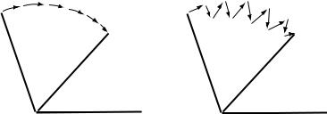
8.3 COORDINATE SPACE FOR OPTIMIZATION

69

(a)

(b)

FIGURE 8.3 Example of paths taken when an angle changes in a geometry optimization. (a) Path taken by an optimization using a Z-matrix or redundant internal coordinates. (b) Path taken by an optimization using Cartesian coordinates.

example, it is very simple for a program to convert a Z-matrix into Cartesian coordinates and then use that space for the geometry optimization.

Many ab initio and semiempirical programs optimize the geometry of the molecule by changing the parameters in the Z-matrix. In general, this can be a very good way to change the geometry because these parameters correspond to molecular motions similar to those seen in the vibrational modes. However, if the geometry is speci®ed in such a way that changing one of the parameters slightly could result in a large distortion to some portion of the molecule, then the geometry optimization is less e½cient. Thus, a poorly constructed Z-matrix can result in a very ine½cient geometry optimization. The construction of Z- matrices is addressed in Chapter 9.

Many computational chemistry programs will do the geometry optimization in Cartesian coordinates. This is often the only way to optimize geometry in molecular mechanics programs and an optional method in orbital-based programs. A Cartesian coordinate optimization may be more e½cient than a poorly constructed Z-matrix. This is often seen in ring systems, where a badly constructed Z-matrix will perform very poorly. Cartesian coordinates can be less e½cient than a well constructed Z-matrix as shown in Figure 8.3. Cartesian coordinates are often preferable when simulating more than one molecule since they allow complete freedom of motion between separate molecules.

In order to have the advantages of a well-constructed Z-matrix, regardless of how the geometry was de®ned, a system called redundant internal coordinates was created. When redundant internal coordinates are used, the input geometry is ®rst converted to a set of Cartesian coordinates. The algorithm then checks the distances between every pair of atoms to determine which are within a reasonable bonding distance. The program then generates a list of atom distances and angles for nearby atoms. This way, the algorithm does the job of constructing a sort of Z-matrix that has more coordinates than are necessary to completely specify the geometry. This is usually the most e½cient way to optimize geometry. The exception is when the automated algorithm did not include a critical coordinate. This can happen with particularly long bonds, such as when the bond is formed or broken in a transition state calculation or inter-