Young - Computational chemistry

110 13 OTHER CHEMICAL PROPERTIES

®nding a molecule that will bind well in a particular binding site requires testing many molecules in many orientations within that site. A de novo program will examine the binding site to determine that it is only reasonable to try molecular orientations in which a nucleophilic group is oriented in a certain way, and so forth.

13.1.8Statistical Processes

It is important to realize that many important processes, such as retention times in a given chromatographic column, are not just a simple aspect of a molecule. These are actually statistical averages of all possible interactions of that molecule and another. These sorts of processes can only be modeled on a molecular level by obtaining many results and then using a statistical distribution of those results. In some cases, group additivities or QSPR methods may be substituted.

13.2MULTIPOLE MOMENTS

The unique multipole moment of a molecule gives a description of the separation of charge of the molecule. Which multipole is unique depends on both the charge and the geometry of the molecule. For a charged ion, the charge, its monopole, is the only unique multipole. The higher-order multipoles, such as the dipole moment, the quadrupole moment, and the like, can still be computed but will be dependent on the origin used for that computation.

Many molecules, such as carbon monoxide, have unique dipole moments. Molecules with a center of inversion, such as carbon dioxide, will have a dipole moment that is zero by symmetry and a unique quadrupole moment. Molecules of Td symmetry, such as methane, have a zero dipole and quadrupole moment and a unique octupole moment. Likewise, molecules of octahedral symmetry will have a unique hexadecapole moment.

Multipole moments are most accurately computed from ab initio calculations. HF calculations with minimal basis sets often give good results. Correlated calculations can yield high-accuracy results. Some semiempirical methods also give reasonable results. For very large molecules, the multipoles can be computed from atomic charges used by molecular mechanics calculations. Computed multipoles can be very sensitive to the geometry at which they are computed, particularly if the value is fairly small in magnitude. It is generally advisable to use multipole moments that were computed with the same level of theory used to optimize the molecular geometry.

13.3FERMI CONTACT DENSITY

The Fermi contact density is de®ned as the electron density at the nucleus of an atom. This is important due to its relationship to analysis methods dependent

13.5 ELECTRON AFFINITY AND IONIZATION POTENTIAL

111

on electron density at the nucleus, such as EPR and NMR spectroscopy. Fermi contact densities are computed with ab initio methods.

13.4 ELECTRONIC SPATIAL EXTENT AND MOLECULAR VOLUME

The electronic spatial extent is a single number that attempts to describe the size of a molecule. This number is computed as the expectation value of electron density times the distance from the center of mass of a molecule. Because the information is condensed down to a single number, it does not distinguish between long chains and more globular molecules.

Molecular volumes are usually computed by a nonquantum mechanical method, which integrates the area inside a van der Waals or Connolly surface of some sort. Alternatively, molecular volume can be determined by choosing an isosurface of the electron density and determining the volume inside of that surface. Thus, one could ®nd the isosurface that contains a certain percentage of the electron density. These properties are important due to their relationship to certain applications, such as determining whether a molecule will ®t in the active site of an enzyme, predicting liquid densities, and determining the cavity size for solvation calculations.

The solvent-excluded volume is a molecular volume calculation that ®nds the volume of space which a given solvent cannot reach. This is done by determining the surface created by running a spherical probe over a hard sphere model of molecule. The size of the probe sphere is based on the size of the solvent molecule.

A convex hull is a molecular surface that is determined by running a planar probe over a molecule. This gives the smallest convex region containing the molecule. It also serves as the maximum volume a molecule can be expected to reach.

13.5ELECTRON AFFINITY AND IONIZATION POTENTIAL

The electron a½nity (EA) and ionization potential (IP) can be computed as the di¨erence between the total energies for the ground state of a molecule and for the ground state of the appropriate ion. The di¨erence between two calculations such as this is often much more accurate than either of the calculations since systematic errors will cancel. Di¨erences of energies from correlated quantum mechanical techniques give very accurate results, often more accurate than might be obtained by experimental methods.

The electron a½nity and ionization potential can be either for vertical excitations or adiabatic excitations. For adiabatic potentials, the geometry of both ions is optimized. For vertical transitions, both energies are computed for the same geometry, optimized for the starting state.

112 13 OTHER CHEMICAL PROPERTIES

Another technique for obtaining an ionization potential is to use the negative of the HOMO energy from a Hartree±Fock calculation. This is called Koopman's theorem; it estimates vertical transitions. This does not apply to methods other than HF but gives a good prediction of the ionization potential for many classes of compounds.

13.6HYPERFINE COUPLING

Traditional wisdom has been that correlated ab initio calculations with large basis sets are necessary to accurately predict hyper®ne coupling constants. More recently, some researchers have begun using the B3LYP functional with a moderate-size basis set (6ÿ31G* or larger). UHF semiempirical calculations were used at one time, but have now been mostly replaced by more accurate methods. The most rigorous calculations include vibronic coupling in order to determine the average of the results for the expected vibrational level occupation at some temperature.

13.7DIELECTRIC CONSTANT

The dielectric constant is a property of a bulk material, not an individual molecule. It arises from the polarity of molecules (static dipole moment), and the polarizability and orientation of molecules in the bulk medium. Often, it is the relative permitivity es that is computed rather than the dielectric constant k, which is the constant of proportionality between the vacuum permitivity e0 and the relative permitivity.

es ˆ ke0

…13:1†

For ¯uids, this is computed by a statistical sampling technique, such as Monte Carlo or molecular dynamics calculations. There are a number of concerns that must be addressed in setting up these calculations, such as

. The choice of boundary conditions

. Whether an adequate sampling of phase space is obtained

. Whether the system size is large enough to represent the bulk material

. Whether the errors in calculation have been estimated correctly

Another way to obtain a relative permitivity is using some simple equations that relate relative permitivity to the molecular dipole moment. These are derived from statistical mechanics. Two of the more well-known equations are the Clausius±Mossotti equation and the Kirkwood equation. These and others are discussed in the review articles referenced at the end of this chapter. The com-

13.9 BIOLOGICAL ACTIVITY

113

putation of dielectric constants is also discussed in the books by Leach, and Allen and Tildesley.

13.8OPTICAL ACTIVITY

Molecular chirality is most often observed experimentally through its optical activity, which is the e¨ect on polarized light. The spectroscopic techniques for measuring optical activity are optical rotary dispersion (ORD), circular dichroism (CD), and vibrational circular dichroism (VCD).

The measurements are predicted computationally with orbital-based techniques that can compute transition dipole moments (and thus intensities) for transitions between electronic states. VCD is particularly di½cult to predict due to the fact that the Born±Oppenheimer approximation is not valid for this property. Thus, there is a choice between using the wave functions computed with the Born±Oppenheimer approximation giving limited accuracy, or very computationally intensive exact computations. Further technical di½culties are encountered due to the gauge dependence of many techniques (dependence on the coordinate system origin).

The most reliable results are obtained using ab initio methods with moderateto large-sized polarized basis sets. The use of gauge-independent atomic orbitals (GIAO) removes gauge dependency problems.

For transition metal complexes, techniques derived from a crystal-®eld theory or ligand-®eld theory description of the molecules have been created. These tend to be more often qualitative than quantitative.

Recent progress in this ®eld has been made in predicting individual atoms' contribution to optical activity. This is done using a wave-functioning, partitioning technique roughly analogous to Mulliken population analysis.

13.9BIOLOGICAL ACTIVITY

There is great commercial interest in predicting the activity of a compound in a biological system. This includes both desired properties, such as drug activity, and undesired properties, such as toxicity. Such a prediction poses some very di½cult problems due to the complexity of biological systems. No method in existence is capable of automatically computing all the interactions between a given molecule and every molecule found in a single cell, let alone an entire organism. Such an attempt is completely beyond the capabilities of any computer hardware available today by many orders of magnitude.

Molecular simulation techniques can be used to predict how a compound will interact with a particular active site of a biological molecule. This is still not trivial because the molecular orientation must be considered along with whether the active site shifts geometry as it approaches.

One very popular technique is to use QSAR. It is, in essence, a curve-®tting

114 13 OTHER CHEMICAL PROPERTIES

technique for creating an equation that predicts biological activity from the properties of the individual molecule only. Once this equation has been created using many compounds of known activity, it can be used to predict the activity of new compounds. QSAR is discussed further in Chapter 30.

Another technique is to use pattern recognition routines. Whereas QSAR relates activity to properties such as the dipole moment, pattern recognition examines only the molecular structure. It thus attempts to ®nd correlations between the functional groups and combinations of functional groups and the biological activity.

Expert systems have also been devised for predicting biological activity. Predicting biological activity is discussed further in Chapter 38.

13.10BOILING POINT AND MELTING POINT

Several methods have been successfully used to predict the normal boiling point of liquids. Group additivity methods give an approximate estimate. Some group additivity methods gain accuracy at the expense of being applicable to a narrow range of chemical systems. Techniques that use a database to parameterize a group additivity method are signi®cantly more accurate.

QSPR methods have yielded the most accurate results. Most often, they use large expansions of parameters obtainable from semiempirical calculations along with other less computationally intensive properties. This is often the method of choice for small molecules.

Molecular dynamics and Monte Carlo simulations can be used, but these methods involve very complex calculations. They are generally only done when more information than just the boiling point is desired and they are not calculations for a novice.

Melting points are much more di½cult to predict accurately. This is because of their dependence on crystal structure. Seemingly similar compounds can have signi®cantly di¨erent melting points due to one geometry being able to pack into a crystal with stronger intermolecular interactions. Some group additivity methods have been designed to give a rough estimate of the melting point.

13.11SURFACE TENSION

Surface tension is usually predicted using group additivity methods for neat liquids. It is much more di½cult to predict the surface tension of a mixture, especially when surfactants are involved. Very large molecular dynamics or Monte Carlo simulations can also be used. Often, it is easier to measure surface tension in the laboratory than to compute it.

13.15 VISUALIZATION 115

13.12VAPOR PRESSURE

Di¨erent compounds can display a very large di¨erence in vapor pressure, depending on what type of intermolecular forces is present. Because of this, di¨erent prediction schemes are used, depending on whether the molecule is nonpolar, polar, or hydrogen-bonding. These methods are usually derived from thermodynamics with an empirical correction factor incorporated. The correction factors usually depend on the type of compound, that is, alcohol, keytone, and, and so forth. These methods are applicable to a wide range of temperatures so long as they are not too close to the temperature at which a phase change occurs. Constants for Henry's law are computed from vapor pressure, log P, and group additivity methods.

13.13SOLUBILITY

A signi®cant amount of research has focused on deriving methods for predicting log P, where P is the octanol±water partition coe½cient. Other solubility and adsorption properties are generally computed from the log P value. There are some group additivity methods for predicting log P, some of which have extremely complex rules. QSPR techniques are reliably applicable to the widest range of compounds. Neural network based methods are very accurate so long as the unknown can be considered an interpolation between compounds in the training set. Database techniques are very accurate for organic compounds. The solvation methods discussed in chapter 24 can also be used.

13.14DIFFUSIVITY

The rate of chemical di¨usion in a non¯owing medium can be predicted. This is usually done with an equation, derived from the di¨usion equation, that incorporates an empirical correction parameter. These correction factors are often based on molar volume. Molecular dynamics simulations can also be used.

Di¨usion in ¯owing ¯uids can be orders of magnitude faster than in non- ¯owing ¯uids. This is generally estimated from continuum ¯uid dynamics simulations.

13.15VISUALIZATION

Data visualization is the process of displaying information in any sort of pictorial or graphic representation. A number of computer programs are available to apply a colorization scheme to data or to work with three-dimensional representations. In recent years, this functionality has been incorporated in many

116 13 OTHER CHEMICAL PROPERTIES

	0.6
	0.5
Ψ	0.4	1s
	0.3
	0.2	2p
	0.1
	0.0

Distance from nucleus (a)

	80
	70
Salary	60
	50
	40
	30
	20
	10
	0

Years employed

(b)

FIGURE 13.1 Graphs that have a one-dimensional data space. (a) Radial portion of the wave function for the hydrogen atom in the 1s ground state and 2p excited state. (b) Hypothetical salary chart.

of the graphic user interface programs used to set up and run chemical calculations. The term ``visualization'' usually refers to the graphic display of numerical results of experimental data, or computational chemistry results, not an artist's representations of the molecule.

13.15.1Coordinate Space

A typical plot of x vs. f …x† is considered to have one coordinate dimension, the x, and one data dimension, f …x†. These data sets are plotted as line graphs, bar graphs, and so forth. These types of plots are readily made with most spreadsheet programs as well as dedicated graphing programs. Figure 13.1 shows two graphs that are considered to have a one-dimensional data space.

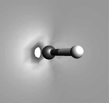
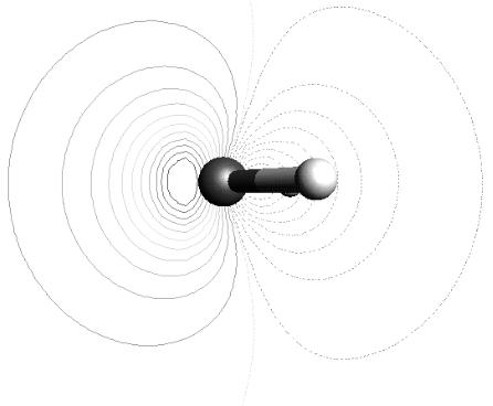
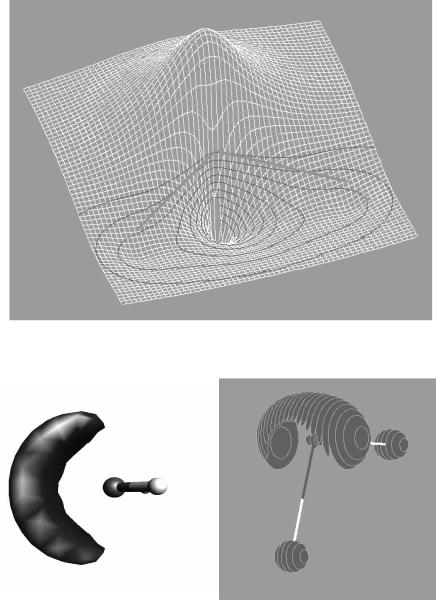
There are also plots that have two coordinate dimensions and one data dimension. Examples of this would be a topographical map or the electron density in one plane. These data sets can be displayed as colorizations (Figure 13.2) or contour plots (Figure 13.3). Colorizations assign a color to each point in the plane according to the value at that point. Contour plots connect all the points having a particular value. Contour plots are perhaps more quantitative in their ability to show the shape of regions with various values. Colorizations are more complete in that no spots are left out. Another technique is to use the third dimension to plot the data values. This is called a mesh plot (Figure 13.4).

Many functions, such as electron density, spin density, or the electrostatic potential of a molecule, have three coordinate dimensions and one data dimension. These functions are often plotted as the surface associated with a particular data value, called an isosurface plot (Figure 13.5). This is the three-dimensional analog of a contour plot.

13.15 VISUALIZATION 117

FIGURE 13.2 Colorizaton of the HOMO-1 orbital of H2O. Colorizations often use a rainbow palette of colors.

13.15.2Data Space

There are ways to plot data with several pieces of data at each point in space. One example would be an isosurface of electron density that has been colorized to show the electrostatic potential value at each point on the surface (Figure 13.6). The shape of the surface shows one piece of information (i.e., the electron density), whereas the color indicates a di¨erent piece of data (i.e., the electrostatic potential). This example is often used to show the nucleophilic and electrophilic regions of a molecule.

Vector quantities, such as a magnetic ®eld or the gradient of electron density, can be plotted as a series of arrows. Another technique is to create an animation showing how the path is followed by a hypothetical test particle. A third technique is to show ¯ow lines, which are the path of steepest descent starting from one point. The ¯ow lines from the bond critical points are used to partition regions of the molecule in the AIM population analysis scheme.

118 13 OTHER CHEMICAL PROPERTIES

FIGURE 13.3 Contour plot of the HOMO-1 orbital of H2O.

One technique for high dimensional data is to reduce the number of dimensions being plotted. For example, one slice of a three-dimensional data set can be plotted with a two-dimensional technique. Another example is plotting the magnitude of vectors rather than the vectors themselves.

13.15.3Software Concerns

The quality of a ®nal image depends on a number of things. Most visualization techniques draw a continuous surface or line by interpolating between data points in the input data. This rendering will be smoother and more accurate if a larger set of input data is used. Most three-dimensional rendering algorithms used in the chemistry ®eld incorporate a smoothing algorithm that assumes surfaces are essentially smooth curves, rather than the disjoint set of points implied by a grid of input data. Figures 13.1 through 13.6 were produced using the default grid sizes, which are usually su½cient to show the shape while minimizing the drain on computational resources. These images were created with the programs UniChem, Spartan, and MOLDEN, all of which are discussed further in Appendix A. A few programs compute the molecular properties from

13.15 VISUALIZATION 119

FIGURE 13.4 Mesh plot of the HOMO-1 orbital of H2O.

(a)

(b)

FIGURE 13.5 Isosurface plots. (a) Region of negative electrostatic potential around the water molecule. (b) Region where the Laplacian of the electron density is negative. Both of these plots have been proposed as descriptors of the lone-pair electrons. This example is typical in that the shapes of these regions are similar, but the Laplacian region tends to be closer to the nucleus.