

Контрольные вопросы
1. К какому типу - прямому или итерационному - относится метод Гаусса?
2. В чем заключается прямой и обратный ход в схеме единственного деления?
3. Как организуется, контроль над вычислениями в прямом и обратном ходе?
4. Как строится итерационная последовательность для нахождения решения системы линейных уравнений?
5. Как формулируется достаточные условия сходимости итерационного процесса?
Лабораторная работа № 4
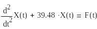
ИССЛЕДОВАНИЕ ДВИЖЕНИЯ УПРУГОЙ СИСТЕМЫ
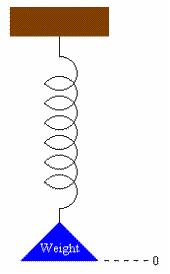
A
spring is attached to a support, the ceiling if you will. A weight
is attached to the end and the spring bobs up and down for a while,
eventually settling down, as shown here.
Consider
a vertical axis whose origin is the weight's position when the
spring is at rest, with the positive axis down. If the spring is set
in vertical motion at time t = 0, the differential equation
describing the spring's position along the vertical axis is given by
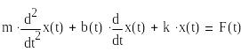
![]()
![]()
where
is
the position of the spring at time t.
is
the mass of the attached weight.
is
a drag coefficient. The term
represents
a retardation of motion that is proportional to velocity. b(t) is
usually a constant reflecting air resistance or friction caused by
the surrounding medium.
is
the spring constant.
is
an external force acting on the spring at time, t.
is
the initial velocity of the spring.
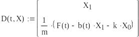
We'll
solve the spring problem as a function of these parameters.
We
use rkfixed
to solve the problem, illustrating some possible types of behavior.
Example
1
![]()
![]()
![]()
![]()
![]()
![]()
![]()
![]()
![]()
![]()
![]()
![]()
![]()
![]()
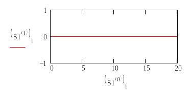
That's
not too exciting . . . but it is correct. With no external force or
initial velocity, the spring never gets started.
Example
2
Here
we'll add a nonzero initial velocity and compute three solutions:
one where the retarding force is 0, one where it is a nonzero
constant, and one where the force is present only for a short time.
![]()
![]()
![]()
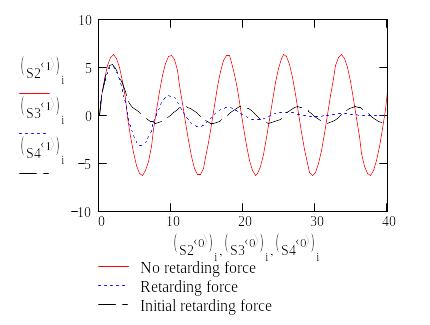
The
three solutions are graphed together below. Note that if there is no
external force and no retarding force, the spring just bounces back
and forth forever. Once the retarding force is added, the motion
decays as you would expect. In the case of the initial retarding
force, the motion is damped at the start but then the spring
oscillates forever.
![]()
![]()
![]()
![]()
Example
3
Now
let's vary the external force factor, keeping the retarding force at
0.
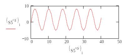
First,
a constant force:
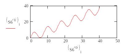
Now,
a steadily increasing force:
![]()
![]()
![]()
![]()
![]()
Keep
in mind, with this example and others where the solution appears
unbounded, the position of the spring is in fact bounded by the
actual length the spring can physically be stretched. The
differential equation does not take this into account and models an
infinitely stretchable spring.
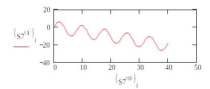
A
steadily increasing force in the opposite direction:
![]()
![]()
![]()
![]()
A
constant force alternating in direction:
By
adjusting the floor
expression in the above example, we can adjust the frequency of the
applied force to be in sync with the frequency of the spring. We
did this here.
![]()
![]()
![]()
![]()
Finally,
a random force :
Лабораторная
работа № 5
Решение
систем ДИФФЕРЕНЦИАЛЬНЫХ уравнений
Consider
the ODE
where
F is defined as
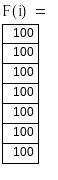
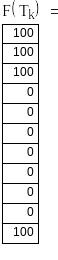
At
integer values F has the value 100, but it is 0 everywhere else:
You
can think of this as a spring problem where at every unit of time a
force of 100 units is applied to the weight at the end of the
spring.
Let's
solve this ODE.
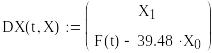
Define:
![]()
![]()
![]()
![]()
![]()
![]()
![]()
![]()
![]()
![]()
![]()
![]()
![]()
![]()
![]()
![]()
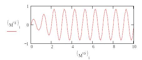
Looks
good, but does it reflect the ODE we're trying to solve? The answer
is no.
Here's why.
We
used a fixed step size routine on the interval
searching
for
points.
This requires a step size of
With
that nice step size and a starting value of 0, you would expect to
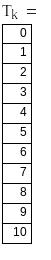
land on an integer value every 20 steps. A look at the time
output reveals![]()
![]()
![]()
![]()
![]()
![]()
So,
this is apparently true.
But,
if we compute F at these values, we see
F
is not 100 at every one of these “integer” values as it should
be!![]()
![]()
![]()
The
culprit here is our old friend round-off
error. A
closer look at the integer values shows that our steps missed some
of the integer values. Very
close, but no cigar!
Thus,
the full effect of our force factor does not appear in the solution
to our ODE.
But,
the real problem here is not so much the round-off error but the
sensitivity of our function, F, to values that are extremely near an
integer.
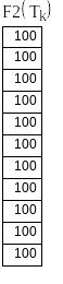
Let's
redefine F,
putting
in a threshold (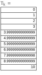
![]()
![]() )
at which we're willing to say something is an integer. Then
)
at which we're willing to say something is an integer. Then
That's
good. Furthermore, our step size of
is
much larger than our threshold. So, while stepping no point will
evaluate to 100 that shouldn't.
Now
let's define
and
solve again:
![]()
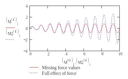
Comparing
the two solutions
we
find that the two solutions agree initially where the force was
being detected in both solutions, but diverge later since the new
solution is feeling the force.
Лабораторная
работа № 6
ИССЛЕДОВАНИЕ
КИНЕМАТИКИ ЭКСКАВАТОРА SmartSketch:
Mathcad-Driven Backhoe Drawing
This
worksheet uses Mathcad to control the position of a backhoe arm in a
SmartSketch drawing.
Note:
This worksheet contains a screenshot of a SmartSketch component. The
working file is located in the CAD\SmrtSkch
subfolder of the Samples
directory.![]()
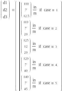
Change
the value of case
to 1, 2, 3, 4 or 5 to control the position of the arm and watch the
drawing automatically update.
![]()

This
program is “globally defined” so that Mathcad recognizes its
existence at the top of the document.
![]()
![]()