

Introduction to 3D Game Programming with DirectX.9.0 - F. D. Luna
.pdf194 Chapter 11
These functions are designed to be flexible and can work with various vertex formats.
HRESULT D3DXComputeBoundingSphere( LPD3DXVECTOR3 pFirstPosition, DWORD NumVertices,
DWORD dwStride, D3DXVECTOR3* pCenter, FLOAT* pRadius
);
pFirstPosition—A pointer to aYvector in the first vertex of an array of vertices that describesLthe position of the vertex
NumVertices—The numberFof vertices in the vertex array
dwStride—The size of each vertex in bytes. This is needed because a vertex structureMmay have additional information such as a normal vector and texture coordinates that is not needed for the bounding sphere function,Aand the function needs to know how much data to Eskip over to get to the next vertex position.
pCenterT—Returns the center of the bounding sphere
pRadius—Returns the radius of the bounding sphere
DWORD dwStride, D3DXVECTOR3* pMin, D3DXVECTOR3* pMax
);
The first three parameters are exactly the same as the first three in D3DXComputeBoundingSphere. The last two parameters are used to return the bounding box’s minimum and maximum point, respectively.
11.4.1 Some New Special Constants
Let’s introduce two constants that prove useful throughout the rest of this book. We add these to the d3d namespace:
namespace d3d
{
...
const float INFINITY = FLT_MAX; const float EPSILON = 0.001f;
The INFINITY constant is simply used to represent the largest number that we can store in a float. Since we can’t have a float bigger than FLT_MAX, we can conceptualize it as infinity, which makes for more readable code that signifies ideas of infinity. The EPSILON
Team-Fly®

Meshes Part II 195
constant is a small value we define such that we consider any number smaller than it equal to zero. This is necessary because due to floatingpoint imprecision, a number that should really be zero may be off slightly. Thus, comparing it to zero would fail. We therefore test if a floating-point variable is zero by testing if it’s less than EPSILON. The following function illustrates how EPSILON can be used to test if two floating-point values are equal:
bool Equals(float lhs, float rhs)
{
// if lhs == rhs their difference should be zero return fabs(lhs - rhs) < EPSILON ? true : false;
}
11.4.2 Bounding Volume Types
To facilitate work with bounding spheres and bounding volumes, it is natural to implement classes representing each. We implement such classes now in the d3d namespace:
struct BoundingBox
{
BoundingBox();
bool isPointInside(D3DXVECTOR3& p);
D3DXVECTOR3 _min; D3DXVECTOR3 _max;
};
struct BoundingSphere
{
BoundingSphere();
D3DXVECTOR3 _center; float _radius;
};
d3d::BoundingBox::BoundingBox()
{
// infinite small bounding box _min.x = d3d::INFINITY; _min.y = d3d::INFINITY; _min.z = d3d::INFINITY;
_max.x = -d3d::INFINITY; _max.y = -d3d::INFINITY; _max.z = -d3d::INFINITY;
}
bool d3d::BoundingBox::isPointInside(D3DXVECTOR3& p)
{
// is the point inside the bounding box?
if(p.x >= _min.x && p.y >= _min.y && p.z >= _min.z &&
P a r t I I I

196 Chapter 11
p.x <= _max.x && p.y <= _max.y && p.z <= _max.z)
{
return true;
}
else
{
return false;
}
}
d3d::BoundingSphere::BoundingSphere()
{
_radius = 0.0f;
}
11.4.3 Sample Application: Bounding Volumes
The Bounding Volumes sample located in this chapter’s folder in the companion files demonstrates using D3DXComputeBoundingSphere and D3DXComputeBoundingBox. The program loads an XFile and computes its bounding sphere and mesh. It then creates two ID3DXMesh objects, one to model the bounding sphere and one to model the bounding box. The mesh corresponding to the XFile is then rendered with either the bounding sphere or bounding box displayed (see Figure 11.5). The user can switch between displaying the bounding sphere and bounding box mesh by pressing the Spacebar.
Figure 11.5: A screen shot of the Bounding Volumes sample. Note that transparency using alpha blending is used to make the bounding sphere transparent.
The sample is pretty straightforward, and we will leave it to you to study the source code. The two functions we implement that are of interest to this discussion compute the bounding sphere and bounding box of a specific mesh:

Meshes Part II 197
bool ComputeBoundingSphere(
ID3DXMesh* mesh, // mesh to compute bounding sphere for d3d::BoundingSphere* sphere) // return bounding sphere
{
HRESULT hr = 0;
BYTE* v = 0; mesh->LockVertexBuffer(0, (void**)&v);
hr = D3DXComputeBoundingSphere( (D3DXVECTOR3*)v, mesh->GetNumVertices(), D3DXGetFVFVertexSize(mesh->GetFVF()), &sphere->_center,
&sphere->_radius);
mesh->UnlockVertexBuffer();
if( FAILED(hr) ) return false;
return true;
}
bool ComputeBoundingBox(
ID3DXMesh* mesh, // mesh to compute bounding box for d3d::BoundingBox* box) // return bounding box
{
HRESULT hr = 0;
BYTE* v = 0; mesh->LockVertexBuffer(0, (void**)&v);
hr = D3DXComputeBoundingBox( (D3DXVECTOR3*)v, mesh->GetNumVertices(),
D3DXGetFVFVertexSize(mesh->GetFVF()), &box->_min,
&box->_max);
mesh->UnlockVertexBuffer();
if( FAILED(hr) ) return false;
return true;
}
Notice that the cast (D3DXVECTOR3*)v assumes the vertex position component is stored first in the vertex structure that we are using. Also notice that we can use the D3DXGetFVFVertexSize function to get the size of a vertex structure given the flexible vertex format description.
P a r t I I I

198Chapter 11
11.5Summary
We can construct complex triangle meshes using 3D modeling programs and either export or convert them to XFiles. Then, using the D3DXLoadMeshFromX function, we can load the mesh data in an XFile into an ID3DXMesh object that we can use in our applications.
Progressive meshes, represented by the ID3DXPMesh interface, can be used to control the level of detail of a mesh; that is, we can adjust the detail of the mesh dynamically. This is useful because we will often want to adjust the detail of the mesh based on how prominent it is in the scene. For example, a mesh closer to the viewer should be rendered with more detail than a mesh far away from the viewer.
We can compute the bounding sphere and bounding box using the
D3DXComputeBoundingSphere and D3DXComputeBoundingBox functions, respectively. Bounding volumes are useful because they approximate the volume of a mesh and can therefore be used to speed up calculations related to the volume of space that a mesh occupies.

Chapter 12
Building a Flexible
Camera Class
Thus far, we have used the D3DXMatrixLookAtLH function to compute a view space transformation matrix. This function is particularly useful for positioning and aiming a camera in a fixed position, but its user interface is not so useful for a moving camera that reacts to user input. This motivates us to develop our own solution. In this chapter we show how to implement a Camera class that gives us better control of the camera than the D3DXMatrixLookAtLH function and is particularly suitable for flight simulators and games played from the firstperson perspective.
Objective
To learn how to implement a flexible Camera class that can be used for flight simulators and games played from the first-person perspective
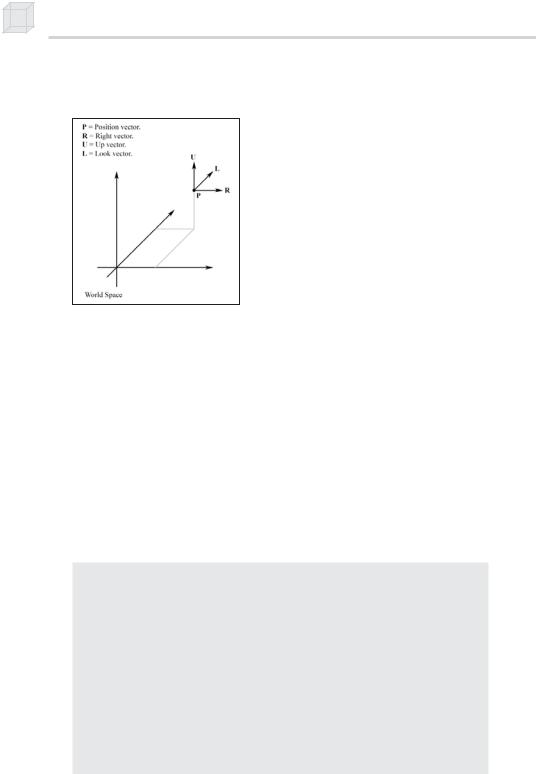
12.1Camera Design
We define the position and orientation of the camera relative to the world coordinate system using four camera vectors: a right vector, up vector, look vector, and position vector, as Figure 12.1 illustrates. These vectors essentially define a local coordinate system for the camera described relative to the world coordinate system. Since the right, up, and look vectors define the camera’s orientation in the world, we sometimes refer to all three as the orientation vectors. The orientation vectors must be orthonormal. A set of vectors is orthonormal if they are mutually perpendicular to each other and of unit length. The reason we make this restriction is because later we insert the orientation vectors into the rows of a matrix, and a matrix where the row vectors are orthonormal means the matrix is orthogonal. Recall that an orthogonal
199
200 Chapter 12
matrix has the property that its inverse equals its transpose. This is useful later in section 12.2.1.2.
Figure 12.1: The camera vectors defining the position and orientation of the camera relative to the world
With these four vectors describing the camera, we would like our camera to be able to perform the following six operations:
Rotate around the right vector (pitch)
Rotate around the up vector (yaw)
Rotate around the look vector (roll)
Strafe along the right vector
Fly along the up vector
Move along the look vector
Through these six operations, we are able to move along three axes and rotate around three axes, giving us a flexible six degrees of freedom. The following Camera class definition reflects our description of data and desired methods:
class Camera
{
public:
enum CameraType { LANDOBJECT, AIRCRAFT };
Camera();
Camera(CameraType cameraType); ~Camera();
void strafe(float units); void fly(float units); void walk(float units);
void pitch(float angle); void yaw(float angle); void roll(float angle);
//left/right
//up/down
//forward/backward
//rotate on right vector
//rotate on up vector
//rotate on look vector

Building a Flexible Camera Class 201
void getViewMatrix(D3DXMATRIX* V);
void setCameraType(CameraType cameraType); void getPosition(D3DXVECTOR3* pos);
void setPosition(D3DXVECTOR3* pos); void getRight(D3DXVECTOR3* right); void getUp(D3DXVECTOR3* up);
void getLook(D3DXVECTOR3* look);
private:
CameraType _cameraType; D3DXVECTOR3 _right; D3DXVECTOR3 _up; D3DXVECTOR3 _look; D3DXVECTOR3 _pos;
};
One thing shown in this class definition that we haven’t discussed is the CameraType enumerated type. Presently, our camera supports two types of camera models, a LANDOBJECT model and an AIRCRAFT model. The AIRCRAFT model allows us to move freely through space and gives us six degrees of freedom. However, in some games, such as a first-person shooter, people can’t fly; therefore we must restrict movement on certain axes. Specifying LANDOBJECT for the camera type has these restrictions carried out, as you can see in the following section.
12.2 Implementation Details
12.2.1 Computing the View Matrix
We now show how the view matrix transformation can be computed
given the camera vectors. Let p = (px, py, pz), r = (rx, ry, rz), u = (ux, uy, uz), and d = (dx, dy, dz) be the position, right, up, and look vectors,
respectively.
Recall that in Chapter 2 we said that the view space transformation transforms the geometry in the world so that the camera is centered at the origin and axis aligned with the major coordinate axes (see Figure 12.2).
P a r t I I I

