- •About the author
- •Brief Contents
- •Contents
- •Preface
- •This Book’s Approach
- •What’s New in the Seventh Edition?
- •The Arrangement of Topics
- •Part One, Introduction
- •Part Two, Classical Theory: The Economy in the Long Run
- •Part Three, Growth Theory: The Economy in the Very Long Run
- •Part Four, Business Cycle Theory: The Economy in the Short Run
- •Part Five, Macroeconomic Policy Debates
- •Part Six, More on the Microeconomics Behind Macroeconomics
- •Epilogue
- •Alternative Routes Through the Text
- •Learning Tools
- •Case Studies
- •FYI Boxes
- •Graphs
- •Mathematical Notes
- •Chapter Summaries
- •Key Concepts
- •Questions for Review
- •Problems and Applications
- •Chapter Appendices
- •Glossary
- •Translations
- •Acknowledgments
- •Supplements and Media
- •For Instructors
- •Instructor’s Resources
- •Solutions Manual
- •Test Bank
- •PowerPoint Slides
- •For Students
- •Student Guide and Workbook
- •Online Offerings
- •EconPortal, Available Spring 2010
- •eBook
- •WebCT
- •BlackBoard
- •Additional Offerings
- •i-clicker
- •The Wall Street Journal Edition
- •Financial Times Edition
- •Dismal Scientist
- •1-1: What Macroeconomists Study
- •1-2: How Economists Think
- •Theory as Model Building
- •The Use of Multiple Models
- •Prices: Flexible Versus Sticky
- •Microeconomic Thinking and Macroeconomic Models
- •1-3: How This Book Proceeds
- •Income, Expenditure, and the Circular Flow
- •Rules for Computing GDP
- •Real GDP Versus Nominal GDP
- •The GDP Deflator
- •Chain-Weighted Measures of Real GDP
- •The Components of Expenditure
- •Other Measures of Income
- •Seasonal Adjustment
- •The Price of a Basket of Goods
- •The CPI Versus the GDP Deflator
- •The Household Survey
- •The Establishment Survey
- •The Factors of Production
- •The Production Function
- •The Supply of Goods and Services
- •3-2: How Is National Income Distributed to the Factors of Production?
- •Factor Prices
- •The Decisions Facing the Competitive Firm
- •The Firm’s Demand for Factors
- •The Division of National Income
- •The Cobb–Douglas Production Function
- •Consumption
- •Investment
- •Government Purchases
- •Changes in Saving: The Effects of Fiscal Policy
- •Changes in Investment Demand
- •3-5: Conclusion
- •4-1: What Is Money?
- •The Functions of Money
- •The Types of Money
- •The Development of Fiat Money
- •How the Quantity of Money Is Controlled
- •How the Quantity of Money Is Measured
- •4-2: The Quantity Theory of Money
- •Transactions and the Quantity Equation
- •From Transactions to Income
- •The Assumption of Constant Velocity
- •Money, Prices, and Inflation
- •4-4: Inflation and Interest Rates
- •Two Interest Rates: Real and Nominal
- •The Fisher Effect
- •Two Real Interest Rates: Ex Ante and Ex Post
- •The Cost of Holding Money
- •Future Money and Current Prices
- •4-6: The Social Costs of Inflation
- •The Layman’s View and the Classical Response
- •The Costs of Expected Inflation
- •The Costs of Unexpected Inflation
- •One Benefit of Inflation
- •4-7: Hyperinflation
- •The Costs of Hyperinflation
- •The Causes of Hyperinflation
- •4-8: Conclusion: The Classical Dichotomy
- •The Role of Net Exports
- •International Capital Flows and the Trade Balance
- •International Flows of Goods and Capital: An Example
- •Capital Mobility and the World Interest Rate
- •Why Assume a Small Open Economy?
- •The Model
- •How Policies Influence the Trade Balance
- •Evaluating Economic Policy
- •Nominal and Real Exchange Rates
- •The Real Exchange Rate and the Trade Balance
- •The Determinants of the Real Exchange Rate
- •How Policies Influence the Real Exchange Rate
- •The Effects of Trade Policies
- •The Special Case of Purchasing-Power Parity
- •Net Capital Outflow
- •The Model
- •Policies in the Large Open Economy
- •Conclusion
- •Causes of Frictional Unemployment
- •Public Policy and Frictional Unemployment
- •Minimum-Wage Laws
- •Unions and Collective Bargaining
- •Efficiency Wages
- •The Duration of Unemployment
- •Trends in Unemployment
- •Transitions Into and Out of the Labor Force
- •6-5: Labor-Market Experience: Europe
- •The Rise in European Unemployment
- •Unemployment Variation Within Europe
- •The Rise of European Leisure
- •6-6: Conclusion
- •7-1: The Accumulation of Capital
- •The Supply and Demand for Goods
- •Growth in the Capital Stock and the Steady State
- •Approaching the Steady State: A Numerical Example
- •How Saving Affects Growth
- •7-2: The Golden Rule Level of Capital
- •Comparing Steady States
- •The Transition to the Golden Rule Steady State
- •7-3: Population Growth
- •The Steady State With Population Growth
- •The Effects of Population Growth
- •Alternative Perspectives on Population Growth
- •7-4: Conclusion
- •The Efficiency of Labor
- •The Steady State With Technological Progress
- •The Effects of Technological Progress
- •Balanced Growth
- •Convergence
- •Factor Accumulation Versus Production Efficiency
- •8-3: Policies to Promote Growth
- •Evaluating the Rate of Saving
- •Changing the Rate of Saving
- •Allocating the Economy’s Investment
- •Establishing the Right Institutions
- •Encouraging Technological Progress
- •The Basic Model
- •A Two-Sector Model
- •The Microeconomics of Research and Development
- •The Process of Creative Destruction
- •8-5: Conclusion
- •Increases in the Factors of Production
- •Technological Progress
- •The Sources of Growth in the United States
- •The Solow Residual in the Short Run
- •9-1: The Facts About the Business Cycle
- •GDP and Its Components
- •Unemployment and Okun’s Law
- •Leading Economic Indicators
- •9-2: Time Horizons in Macroeconomics
- •How the Short Run and Long Run Differ
- •9-3: Aggregate Demand
- •The Quantity Equation as Aggregate Demand
- •Why the Aggregate Demand Curve Slopes Downward
- •Shifts in the Aggregate Demand Curve
- •9-4: Aggregate Supply
- •The Long Run: The Vertical Aggregate Supply Curve
- •From the Short Run to the Long Run
- •9-5: Stabilization Policy
- •Shocks to Aggregate Demand
- •Shocks to Aggregate Supply
- •10-1: The Goods Market and the IS Curve
- •The Keynesian Cross
- •The Interest Rate, Investment, and the IS Curve
- •How Fiscal Policy Shifts the IS Curve
- •10-2: The Money Market and the LM Curve
- •The Theory of Liquidity Preference
- •Income, Money Demand, and the LM Curve
- •How Monetary Policy Shifts the LM Curve
- •Shocks in the IS–LM Model
- •From the IS–LM Model to the Aggregate Demand Curve
- •The IS–LM Model in the Short Run and Long Run
- •11-3: The Great Depression
- •The Spending Hypothesis: Shocks to the IS Curve
- •The Money Hypothesis: A Shock to the LM Curve
- •Could the Depression Happen Again?
- •11-4: Conclusion
- •12-1: The Mundell–Fleming Model
- •The Goods Market and the IS* Curve
- •The Money Market and the LM* Curve
- •Putting the Pieces Together
- •Fiscal Policy
- •Monetary Policy
- •Trade Policy
- •How a Fixed-Exchange-Rate System Works
- •Fiscal Policy
- •Monetary Policy
- •Trade Policy
- •Policy in the Mundell–Fleming Model: A Summary
- •12-4: Interest Rate Differentials
- •Country Risk and Exchange-Rate Expectations
- •Differentials in the Mundell–Fleming Model
- •Pros and Cons of Different Exchange-Rate Systems
- •The Impossible Trinity
- •12-6: From the Short Run to the Long Run: The Mundell–Fleming Model With a Changing Price Level
- •12-7: A Concluding Reminder
- •Fiscal Policy
- •Monetary Policy
- •A Rule of Thumb
- •The Sticky-Price Model
- •Implications
- •Adaptive Expectations and Inflation Inertia
- •Two Causes of Rising and Falling Inflation
- •Disinflation and the Sacrifice Ratio
- •13-3: Conclusion
- •14-1: Elements of the Model
- •Output: The Demand for Goods and Services
- •The Real Interest Rate: The Fisher Equation
- •Inflation: The Phillips Curve
- •Expected Inflation: Adaptive Expectations
- •The Nominal Interest Rate: The Monetary-Policy Rule
- •14-2: Solving the Model
- •The Long-Run Equilibrium
- •The Dynamic Aggregate Supply Curve
- •The Dynamic Aggregate Demand Curve
- •The Short-Run Equilibrium
- •14-3: Using the Model
- •Long-Run Growth
- •A Shock to Aggregate Supply
- •A Shock to Aggregate Demand
- •A Shift in Monetary Policy
- •The Taylor Principle
- •14-5: Conclusion: Toward DSGE Models
- •15-1: Should Policy Be Active or Passive?
- •Lags in the Implementation and Effects of Policies
- •The Difficult Job of Economic Forecasting
- •Ignorance, Expectations, and the Lucas Critique
- •The Historical Record
- •Distrust of Policymakers and the Political Process
- •The Time Inconsistency of Discretionary Policy
- •Rules for Monetary Policy
- •16-1: The Size of the Government Debt
- •16-2: Problems in Measurement
- •Measurement Problem 1: Inflation
- •Measurement Problem 2: Capital Assets
- •Measurement Problem 3: Uncounted Liabilities
- •Measurement Problem 4: The Business Cycle
- •Summing Up
- •The Basic Logic of Ricardian Equivalence
- •Consumers and Future Taxes
- •Making a Choice
- •16-5: Other Perspectives on Government Debt
- •Balanced Budgets Versus Optimal Fiscal Policy
- •Fiscal Effects on Monetary Policy
- •Debt and the Political Process
- •International Dimensions
- •16-6: Conclusion
- •Keynes’s Conjectures
- •The Early Empirical Successes
- •The Intertemporal Budget Constraint
- •Consumer Preferences
- •Optimization
- •How Changes in Income Affect Consumption
- •Constraints on Borrowing
- •The Hypothesis
- •Implications
- •The Hypothesis
- •Implications
- •The Hypothesis
- •Implications
- •17-7: Conclusion
- •18-1: Business Fixed Investment
- •The Rental Price of Capital
- •The Cost of Capital
- •The Determinants of Investment
- •Taxes and Investment
- •The Stock Market and Tobin’s q
- •Financing Constraints
- •Banking Crises and Credit Crunches
- •18-2: Residential Investment
- •The Stock Equilibrium and the Flow Supply
- •Changes in Housing Demand
- •18-3: Inventory Investment
- •Reasons for Holding Inventories
- •18-4: Conclusion
- •19-1: Money Supply
- •100-Percent-Reserve Banking
- •Fractional-Reserve Banking
- •A Model of the Money Supply
- •The Three Instruments of Monetary Policy
- •Bank Capital, Leverage, and Capital Requirements
- •19-2: Money Demand
- •Portfolio Theories of Money Demand
- •Transactions Theories of Money Demand
- •The Baumol–Tobin Model of Cash Management
- •19-3 Conclusion
- •Lesson 2: In the short run, aggregate demand influences the amount of goods and services that a country produces.
- •Question 1: How should policymakers try to promote growth in the economy’s natural level of output?
- •Question 2: Should policymakers try to stabilize the economy?
- •Question 3: How costly is inflation, and how costly is reducing inflation?
- •Question 4: How big a problem are government budget deficits?
- •Conclusion
- •Glossary
- •Index
A P P E N D I X
The Large Open Economy
When analyzing policy for a country such as the United States, we need to combine the closed-economy logic of Chapter 3 and the small-open-economy logic of this chapter. This appendix presents a model of an economy between these two extremes, called the large open economy.
Net Capital Outflow
The key difference between the small and large open economies is the behavior of the net capital outflow. In the model of the small open economy, capital flows freely into or out of the economy at a fixed world interest rate r *. The model of the large open economy makes a different assumption about international capital flows. To understand this assumption, keep in mind that the net capital outflow is the amount that domestic investors lend abroad minus the amount that foreign investors lend here.
Imagine that you are a domestic investor—such as the portfolio manager of a university endowment—deciding where to invest your funds. You could invest domestically (for example, by making loans to U.S. companies), or you could invest abroad (by making loans to foreign companies). Many factors may affect your decision, but surely one of them is the interest rate you can earn. The higher the interest rate you can earn domestically, the less attractive you would find foreign investment.
Investors abroad face a similar decision. They have a choice between investing in their home country and lending to someone in the United States. The higher the interest rate in the United States, the more willing foreigners are to lend to U.S. companies and to buy U.S. assets.
Thus, because of the behavior of both domestic and foreign investors, the net flow of capital to other countries, which we’ll denote as CF, is negatively related to the domestic real interest rate r. As the interest rate rises, less of our saving flows abroad, and more funds for capital accumulation flow in from other countries. We write this as
CF = CF(r).
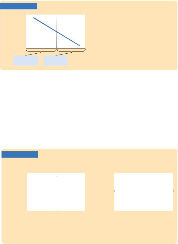
This equation states that the net capital outflow is a function of the domestic interest rate. Figure 5-15 illustrates this relationship. Notice that CF can be either positive or negative, depending on whether the economy is a lender or borrower in world financial markets.
To see how this CF function relates to our previous models, consider Figure 5-16. This figure shows two special cases: a vertical CF function and a horizontal CF function.
153
154 | P A R T I I Classical Theory: The Economy in the Long Run
FIGURE 5-15 |
Real interest |
rate, r |
0 |
|
Net capital |
Borrow from |
Lend to abroad outflow, CF |
abroad (CF < 0) |
(CF > 0) |
How the Net Capital Outflow Depends on the Interest Rate A higher domestic interest rate discourages domestic investors from lending abroad and encourages foreign investors to lend here.
Therefore, net capital outflow CF is negatively related to the interest rate.
The closed economy is the special case shown in panel (a) of Figure 5-16. In the closed economy, there is no international borrowing or lending, and the interest rate adjusts to equilibrate domestic saving and investment. This means that CF = 0 at all interest rates. This situation would arise if investors here and abroad were unwilling to hold foreign assets, regardless of the return. It might also arise if the government prohibited its citizens from transacting in foreign financial markets, as some governments do.
The small open economy with perfect capital mobility is the special case shown in panel (b) of Figure 5-16. In this case, capital flows freely into and out of the country at the fixed world interest rate r*. This situation would arise if investors here and abroad bought whatever asset yielded the highest return and if this economy were
FIGURE 5-16
|
(a) The Closed Economy |
|
|
(b) The Small Open Economy With |
||
|
|
|
Perfect Capital Mobility |
|||
Real interest |
|
Real interest |
|
|
||
|
|
|||||
rate, r |
|
|
rate, r |
|
|
|
|
|
|
r* |
|
|
|
|
|
|
|
|
|
|
|
|
|
|
|
|
|
|
|
|
|
|
|
|
0 |
Net capital |
0 |
Net capital |
|
outflow, CF |
|
outflow, CF |
Two Special Cases In the closed economy, shown in panel (a), the net capital outflow is zero for all interest rates. In the small open economy with perfect capital mobility, shown in panel (b), the net capital outflow is perfectly elastic at the world interest rate r*.
C H A P T E R 5 The Open Economy | 155
too small to affect the world interest rate. The economy’s interest rate would be fixed at the interest rate prevailing in world financial markets.
Why isn’t the interest rate of a large open economy such as the United States fixed by the world interest rate? There are two reasons. The first is that the United States is large enough to influence world financial markets. The more the United States lends abroad, the greater is the supply of loans in the world economy, and the lower interest rates become around the world. The more the United States borrows from abroad (that is, the more negative CF becomes), the higher are world interest rates. We use the label “large open economy” because this model applies to an economy large enough to affect world interest rates.
There is, however, a second reason the interest rate in an economy may not be fixed by the world interest rate: capital may not be perfectly mobile. That is, investors here and abroad may prefer to hold their wealth in domestic rather than foreign assets. Such a preference for domestic assets could arise because of imperfect information about foreign assets or because of government impediments to international borrowing and lending. In either case, funds for capital accumulation will not flow freely to equalize interest rates in all countries. Instead, the net capital outflow will depend on domestic interest rates relative to foreign interest rates. U.S. investors will lend abroad only if U.S. interest rates are comparatively low, and foreign investors will lend in the United States only if U.S. interest rates are comparatively high. The large-open-economy model, therefore, may apply even to a small economy if capital does not flow freely into and out of the economy.
Hence, either because the large open economy affects world interest rates, or because capital is imperfectly mobile, or perhaps for both reasons, the CF function slopes downward. Except for this new downward-sloping CF function, the model of the large open economy resembles the model of the small open economy. We put all the pieces together in the next section.
The Model
To understand how the large open economy works, we need to consider two key markets: the market for loanable funds (where the interest rate is determined) and the market for foreign exchange (where the exchange rate is determined). The interest rate and the exchange rate are two prices that guide the allocation of resources.
The Market for Loanable Funds An open economy’s saving S is used in two ways: to finance domestic investment I and to finance the net capital outflow CF. We can write
S = I + CF.
Consider how these three variables are determined. National saving is fixed by the level of output, fiscal policy, and the consumption function. Investment and net capital outflow both depend on the domestic real interest rate. We can write
_
S = I(r) + CF(r).
156 | P A R T I I Classical Theory: The Economy in the Long Run
FIGURE 5-17
Real interest |
S |
rate, r |
Equilibrium real interest
rate +
I(r) CF(r)
Loanable funds, S, I + CF
The Market for Loanable Funds in the Large Open Economy At the equilibrium interest rate, the supply of loanable funds from saving S balances the demand for loanable funds from domestic investment I and capital investments abroad CF.
Figure 5-17 shows the market for loanable funds. The supply of loanable funds is national saving. The demand for loanable funds is the sum of the demand for domestic investment and the demand for foreign investment (net capital outflow). The interest rate adjusts to equilibrate supply and demand.
The Market for Foreign Exchange Next, consider the relationship between the net capital outflow and the trade balance. The national income accounts identity tells us
NX = S − I.
Because NX is a function of the real exchange rate, and because CF = S − I, we can write
NX(e) = CF.
Figure 5-18 shows the equilibrium in the market for foreign exchange. Once again, the real exchange rate is the price that equilibrates the trade balance and the net capital outflow.
The last variable we should consider is the nominal exchange rate. As before, the nominal exchange rate is the real exchange rate times the ratio of the price levels:
e = e × (P */P).
FIGURE 5-18
Real exchange |
CF |
|
rate, e |
||
|
||
Equilibrium |
|
|
real exchange |
NX(e) |
|
rate |
||
|
|
Net exports, NX
The Market for Foreign-Currency Exchange in the Large Open Economy At the equilibrium exchange rate, the supply of dollars from the net capital outflow, CF, balances the demand for dollars from our net exports of goods and services, NX.