Lecture Notes: Introduction to Finite Element Method

Chapter 5. Plate and Shell Elements

II. Plate Elements

Kirchhoff Plate Elements:

4-Node Quadrilateral Element

z y

Mid surface	4	3

x

1

t

2

w1

∂w

∂w

∂w

∂w

,

,

w2 ,

,

∂x 1

∂y

1

∂x 2

∂y 2

DOF at each node:

w,

∂w

,

∂w

.

∂y

∂y

On each element, the deflection w(x,y) is represented by

	4			∂w			∂w
	w(x, y) = ∑ Ni wi		+ N xi (		)i	+ N yi (		)i	,
				∂x			∂y
	i =1

where Ni, Nxi and Nyi are shape functions. This is an incompatible element! The stiffness matrix is still of the form

k = ∫BT EBdV ,

V

where B is the strain-displacement matrix, and E the stressstrain matrix.

© 1997-2002 Yijun Liu, University of Cincinnati

129

Lecture Notes: Introduction to Finite Element Method

Chapter 5. Plate and Shell Elements

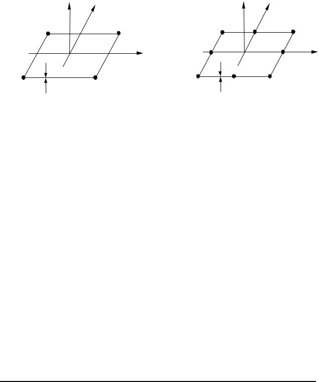
Mindlin Plate Elements:

4-Node Quadrilateral		8-Node Quadrilateral
z	y			z	y
4	3		4	7	3
	x		8		6
					x
1	2	1	t	5	2
t

DOF at each node:	w, θx and θy.
On each element:
n
w(x, y) = ∑Ni wi ,
i=1

n

θx (x, y) = ∑Niθxi ,

i=1

n

θy (x, y) = ∑Niθyi .

i=1

•Three independent fields.

•Deflection w(x,y) is linear for Q4, and quadratic for Q8.

© 1997-2002 Yijun Liu, University of Cincinnati

130

Lecture Notes: Introduction to Finite Element Method

Chapter 5. Plate and Shell Elements

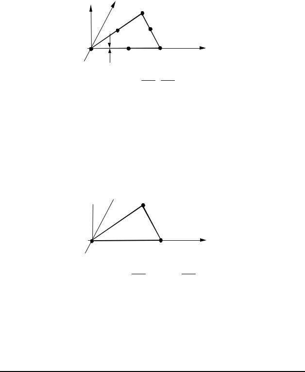
Discrete Kirchhoff Element:

Triangular plate element (not available in ANSYS). Start with a 6-node triangular element,

z	y	3
4		6
1	5	2	x
t

DOF at corner nodes: w,∂∂wx ,∂∂wy ,θx ,θy ;

DOF at mid side nodes: θx ,θy .

Total DOF = 21.

Then, impose conditions γ xz = γ yz = 0, etc., at selected nodes to reduce the DOF (using relations in (15)). Obtain:

z y 3

1	2	x

At each node: w,θx = ∂∂wx ,θy = ∂∂wy .

Total DOF = 9 (DKT Element).

•Incompatible w(x,y); convergence is faster (w is cubic along each edge) and it is efficient.

© 1997-2002 Yijun Liu, University of Cincinnati

131