of atherosclerosis (Fig. 7). However, the elastic modulus is not significantly different from the control artery until the highest grade of atherosclerosis. On the other hand, there appears a significant increase in the arterial stiffness in the grade II atherosclerosis, which is attributable to the wall thickening. Significantly increased calcification and intimal hyperplasia are observed in the wall of the grade III atherosclerosis. From these results, it is concluded that the progression of atherosclerosis induces wall thickening, followed by wall stiffening. However, even if atherosclerosis is advanced, there is essentially no change in the elastic modulus of wall material unless considerable calcification occurs in the wall. Calcified aortas have high elastic moduli. At the most advanced stage of atherosclerosis, the arterial wall has high structural and material stiffness due to calcification and wall hypertrophy (16).

BIBLIOGRAPHY

Cited References

1.Hayashi K, et al. Techniques in the Determination of the Mechanical Properties and Constitutive Laws of Arterial

Walls. In: Leondes C, editor. Cardiovascular Techniques – Biomechanical Systems: Techniques and Applications Vol. II. Boca Raton (FL): CRC Press; 2001. p 6-1–6-61.

2.Hayashi K, Mori K, Miyazaki H. Biomechanical response of femoral vein to chronic elevation of blood pressure in rabbits. Am J Physiol 2003;284:H511–H518.

3.Hayashi K, Nakamura T. Implantable miniature ultrasonic sensors for the measurement of blood flow. Automedica 1989;12:53–62.

4.Abe H, Hayashi K, Sato M, editors. Data Book on Mechanical Properties of Living Cells, Tissues, and Organs. Tokyo: Springer-Verlag; 1996. p 25–125.

5.Fung YC. Biomechanics: Mechanical Properties of Living Tissues. New York: Springer-Verlag; 1993. p 242–320.

6.Hayashi K, et al. Stiffness and elastic behavior of human intracranial and extracranial arteries. J Biomech 1980;13: 175–184.

7.Hayashi K. Mechanical Properties of Soft Tissues and Arterial Walls. In: Holzapfel G, Ogden RW, editors. Biomechanics of Soft Tissue in Cardiovascular Systems. (CISM Courses and Lectures No. 441), Wien: Springer-Verlag; 2003. p 15–64.

8.Hudetz AG. Incremental elastic modulus for orthotropic incompressible arteries. J Biomech 1979;12:651–655.

9.Vaishnav RN, Young JT, Patel DJ. Distribution of stresses an strain energy density through the wall thickness in a canine aortic segment. Circ Res 1973;32:577–583.

10.Chuong CJ, Fung YC. Three-dimensional stress distribution in arteries. Trans ASME J Biomech Eng 1983;105:268–274.

11.Takamizawa K, Hayashi K. Strain energy density function and uniform strain hypothesis for arterial mechanics. J Biomech 1987;20:7–17.

12.Hayashi K, Igarashi Y, Takamizawa K. Mechanical properties and hemodynamics in coronary arteries. In: Kitamura K, Abe H, Sagawa K, editors. New Approaches in Cardiac Mechanics. New York: Gordon and Breach; 1986. p 285–294.

13.Hayashi K. Experimental approaches on measuring the mechanical properties and constitutive laws of arterial walls. Trans ASME J Biomech Eng 1993;115:481–488.

14.Humphrey JD. Cardiovascular Solid Mechanics: Cells, Tissues, and Organs. New York: Springer-Verlag; 2002. p 365–386.

AUDIOMETRY 91

15.Matsumoto T, Hayashi K. Response of arterial wall to hypertension and residual stress. In: Hayashi K, Kamiya A, Ono K, editors. Biomechanics: Functional Adaptation and Remodeling. Tokyo: Springer-Verlag; 1996. p 93–119.

16.Hayashi K, Ide K, Matsumoto T. Aortic walls in atherosclerotic rabbits -Mechanical study. Trans ASME J Biomech Eng 1994;116:284–293.

See also BLOOD PRESSURE, AUTOMATIC CONTROL OF; BLOOD RHEOLOGY;

CUTANEOUS BLOOD FLOW, DOPPLER MEASUREMENT OF; HEMODYNAMICS;

INTRAAORTIC BALLOON PUMP; TONOMETRY, ARTERIAL.

ASSISTIVE DEVICES FOR THE DISABLED. See

ENVIRONMENTAL CONTROL.

ATOMIC ABSORPTION SPECTROMETRY. See

FLAME ATOMIC EMISSION SPECTROMETRY AND ATOMIC ABSORPTION

SPECTROMETRY.

AUDIOMETRY

THOMAS E. BORTON

BETTIE B. BORTON

Auburn University Montgomery

Montgomery, Alabama

JUDITH T. BLUMSACK

Disorders Auburn University

Auburn, Alabama

INTRODUCTION

Audiology is, literally, the science of hearing. In many countries around the world, audiology is a scientific discipline practiced by audiologists. According to the American Academy of Audiology, ‘‘an audiologist is a person who, by virtue of academic degree, clinical training, and license to practice and/or professional credential, is uniquely qualified to provide a comprehensive array of professional services related to the prevention of hearing loss and the audiologic identification, assessment, diagnosis, and treatment of persons with impairment of auditory and vestibular function, as well as the prevention of impairments associated with them. Audiologists serve in a number of roles including clinician, therapist, teacher, consultant, researcher and administrator’’ (1).

An important tool in the practice of audiology is audiometry, which is the measurement of hearing. In general, audiometry entails one or more procedures wherein precisely defined auditory stimuli are presented to the listener in order to elicit a measurable behavioral or physiologic response. Frequently, the term audiometry refers to procedures used in the assessment of an individual’s threshold of hearing for sinusoidal (pure tones) or speech stimuli (2). So-called conventional audiometry is conducted with a calibrated piece of electronic instrumentation called an audiometer to deliver controlled auditory signals to a listener. Currently, however, an expanded definition of audiometry also includes procedures for measuring various physiological and behavioral responses to the presentation

92 ARTERIES, ELASTIC PROPERTIES OF

of auditory stimuli, whether or not the response involves cognition. More sophisticated procedures and equipment are increasingly used to look beyond peripheral auditory structures in order to assess sound processing activity in the neuroauditory system.

Today, audiologists employ audiometric procedures and equipment to assess the function of the auditory system from external ear to brain cortex and serve as consultants to medical practitioners, education systems, the corporate and legal sectors, and government institutions such as the Department of Veterans Affairs. Audiologists also use audiometric procedures to identify and define auditory system function as a basis for nonmedical intervention with newborns, young children with auditory processing disorders, and adults who may require sophisticated amplification systems to develop or maintain their communication abilities and quality of life.

The purpose of this chapter is to acquaint the reader with the basic anatomy of the auditory system, describe some of the instrumentation and procedures currently used for audiometry, and briefly discuss the application of audiometric procedures for the assessment of hearing.

AUDIOMETRY AND ITS ORIGINS

Audiometry refers broadly to qualitative and quantitative measures of auditory function/dysfunction, often with an emphasis on the assessment of hearing loss. It is an important tool in the practice of audiology, a healthcare specialty concerned with the study of hearing, and the functional assessment, diagnosis, and (re)habilitation of hearing impairment. The profession sprang from otology and speech pathology in the 1920s, about the same time that instrumentation for audiometry was being developed. Audiometry grew rapidly in the 1940s when World War II veterans returned home with hearing impairment related to military service (3). Hearing evaluation, the provision of hearing aids, and auditory rehabilitation were pioneered in the Department of Veterans Affairs and, subsequently, universities began programs to educate and train audiologists for service to children and adults in clinics, hospitals, research laboratories and academic settings, and private practice. Audiometry is now a fundamental component of assessing and treating persons with hearing impairment.

Audiometers

Audiometers are electroacoustic instruments designed to meet internationally accepted audiometric performance standards for valid and reliable assessment of hearing sensitivity and auditory processing capability under controlled acoustic conditions. The audiometer was first described around the turn of the twentieth century (4) and was used mainly in laboratory research at the University of Iowa. A laboratory assistant at the university, C. C. Bunch, would later publish a classic textbook describing audiometric test results in patients with a variety of hearing disorders (5). The first commercial audiometer, called the Western Electric 1A, was developed in the early 1920s by the Bell Telephone Laboratories in the United States, and was described by Fowler and Wegel in 1922 (6). More

than 20 years elapsed before the use of audiometers for hearing assessment was widely recognized (7), and it was not until the early 1950s (8) that audiometry became an accepted clinical practice. Since that time, electroacoustic instrumentation for audiometry has been described in standards written by scientists and experts designed to introduce uniformity and facilitate the international exchange of data and test results. The American National Standards Institute (ANSI), the International Standards Organization (ISO), and the International Electrotechnical Commission (IEC) are recognized bodies that have developed accepted standards for equipment used in audiometry and in psychophysical measurement, acoustics, and research. In the present day, audiometric procedures are routinely used throughout the world for identifying auditory dysfunction in newborns, assessing hearing disorders associated with ear disease, and monitoring the hearing of patients at risk for damage to the auditory system (e.g., because of exposure to hazardous noise, toxic substances).

Types of Audiometers

In the United States, ANSI (9) classifies audiometers according to several criteria, including the use for which they are designed, how they are operated, the signals they produce, their portability, and other factors.

In general, Type IV screening audiometers (designed to differentiate those with normal hearing sensitivity from those with hearing impairment) are of simpler design than those instruments used for in-depth diagnostic evaluation for medical purposes (Type I audiometers). There are automatic and computer-processor audiometers (Bekesy or self-recording types), extended high-frequency (Type HF), free-field equivalent audiometers (Type E), speech audiometers (Types A, B, and C depending on available features), and others for specific purposes.

Audiometers possess one or more oscillation networks to generate pure tones of differing frequencies, switching networks to interrupt and direct stimuli, and attenuating systems calibrated in decibels (dB) relative to audiometric zero. The intensity range for most attenuation networks usually approximates 100 dB, typically graduated in steps of 5 dB. The ‘‘zero dB’’ level represents normal hearing sensitivity across the test frequency range for young adults under favorable, noise-free laboratory conditions. Collection of these hearing level reference data from different countries began in the 1950s and 1960s. These reference levels have been accepted by internationally recognized standards organizations. Audiometers also include various types of output transducers for presentation of signals to the listener, including earphones, bone-conduction vibrators, and loudspeakers. As the audiometrically generated signals are affected substantially by the electroacoustic characteristics of these devices (e.g., frequency response), versatile audiometers have multiple calibrated output networks to facilitate switching between transducers depending on the clinical application of interest.

Figure 1 shows the general layout of a Type I diagnostic audiometer. Such instruments are required by standards governing them to produce a stable output at a range of

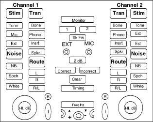
Figure 1. Typical diagnostic audiometer.

operating temperatures and humidity and meet a wide variety of electrical and other safety standards, in addition to precise electroacoustic standards for frequency, intensity, spectral purity, maximum output sound pressure level (SPL), and harmonic distortion. Type II audiometers have fewer required features and less flexibility, and Type IV audiometers have even more limitations.

Audiometric Calibration

To ensure that an audiometer is performing in accordance with the relevant standard, the instrument’s electroacoustic characteristics are checked and adjusted as necessary, usually following a routine procedure. These calibration activities may be conducted at the manufacturing facility or an outside laboratory, but are most often accomplished on site at least annually. Calibration of speakers in a sound field is typically conducted on site because the unique acoustic characteristics of a specific field cannot easily be reproduced in a remote calibration facility.

Calibration of audiometers is routinely checked using instruments such as oscilloscopes, multimeters, spectrometers, and sound-level meters to verify frequency, intensity, and temporal characteristics of the equipment. Output transducers such as earphones and bone stimulators can be calibrated in two ways: (1) using ‘‘real ear’’ methods, involving individuals or groups of persons free from ear pathology and who meet other criteria, or (2) using hard-walled couplers (artificial ears) and pressure transducers specified by the relevant standard.

Audiometric Standards

Electroacoustic instrumentation for audiometry has been described in national and international standards written by scientists and experts designed to introduce uniformity and facilitate the international exchange of data and test results. ANSI, ISO, and IEC are recognized bodies that have developed accepted standards for equipment used in audiometry and acoustics. Some standards relate to equipment, others to audiometric procedures, and still others to

AUDIOMETRY 93

the environment and conditions in which audiometry should be conducted (10).

The aim of standards for audiometric equipment and procedures is to assure precision of equipment functions to help ensure that test results can be interpreted meaningfully and reliably within and between clinics and laboratories using different equipment and personnel in various geographical locations. The results of audiometry often help to provide a basis for decisions regarding intervention strategies, such as medical or surgical intervention, referral for cochlear implantation, hearing aid selection and fitting, application of assistive listening devices, or selection of appropriate educational or vocational placement. As in any measurement scheme, audiometric test results can be no more precise than the function of the equipment and the procedures with which those measurements are made.

PURE TONE AUDIOMETRY

Psychophysical Methods

Audiometry may be conducted with a variety of methodologies depending on the goal of the procedure and subject variables such as age, mental status, and motivation. For example, the hearing sensitivity of very young children may be estimated by assessing the effects of auditory stimuli presented in a sound field on startle-type reflexes, level of arousal, and localization. Patients who are developmentally delayed may be taught with reinforcement to push a button upon presentation of a test stimulus. Children of preschool age may be taught to make a motor response to auditory test stimuli using play audiometric techniques.

In conventional audiometry, auditory stimuli are presented through special insert or supra-aural earphones, or a bone oscillator worn by the patient. When indicated, a sound field around the listener may be created by presenting stimuli through strategically placed loudspeakers. Most threshold audiometric tests in school-aged children and adults can be conducted using one of two psychophysical methods originally developed by Gustav Fechner: (1) the method of adjustment, or (2) the method of limits (11). In the method of adjustment, the intensity of an auditory stimulus is adjusted by the listener according to some criterion (just audible or just inaudible), usually across a range of continuously or discretely adjusted frequencies. Nobel Prize Laureate Georg von Bekesy initially introduced this methodology into the practice of audiometry in 1947 (12). With this approach, listeners heard sinusoidal stimuli that changed from lower to higher test frequencies, and adjusted the intensity of continuous and interrupted tones from ‘‘just inaudible’’ to ‘‘just audible’’. As shown in Fig. 2, this methodology yielded information about the listener’s auditory threshold throughout the test frequency range. The relationship of threshold tracings for the pulsed and continuous stimuli added additional information about the site of lesion causing the hearing loss (13,14).

Later, it was found that the tracing patterns tracked by hearing-impaired patients at their most comfortable loudness levels, instead of their threshold levels, yielded additional useful diagnostic information (15). A myriad of

94 AUDIOMETRY

Figure 2. Bekesy audiometric tracing of continuous and interrupted tones around auditory threshold.

factors associated with this psychophysical measurement method, including the age of the listener, learning effects, and the length of time required to obtain stable test results, make these methods unsuitable for routine diagnostic purposes, especially in young children. Nevertheless, audiometers incorporating this methodology are manufactured to precise specifications (9) and are routinely used in hearing conservation programs to record the auditory sensitivity of large numbers of employees working in industrial or military settings.

In most clinical situations today, routine threshold audiometry is conducted using the method of limits. In this approach, the examiner adjusts the intensity of the auditory stimuli of various frequencies according to a predetermined schema, and the listener responds with a gross motor act (such as pushing a button or raising a hand) when the stimulus is detected. Although auditory threshold may be estimated using a variety of procedural variants (ascending, descending, mixed, adaptive), research has established (16) that an ascending approach in which tonal stimuli are presented to the listener from inaudible intensity to a just audible level is a valid and reliable approach for cooperative and motivated listeners, and the technique most parsimonious with clinical time and effort. In this approach, tonal stimuli are presented at intensity levels below the listener’s threshold of audibility and raised in increments until a response is obtained. At this point, the intensity is lowered below the response level and increased incrementally until a response is obtained. When the method of limits is used, auditory threshold is typically defined as the lowest intensity level that elicits a reliable response from the patient on approximately 50% or more of these ‘‘ascending’’ trials.

Sound Pathways of the Auditory System

The fundamental anatomy of the ear is depicted in Fig. 3. Sound enters the auditory mechanism by two main routes, air conduction and bone conduction. Most speech and other sounds in the ambient environment enter the ear by air conduction. The outer ear collects and funnels sound waves into the ear canal, provides a small amount of amplification

Figure 3. Anatomy of the peripheral auditory mechanism. Adapted from medical illustrations by NIH, Medical Arts & Photography Branch.

to auditory signals, and conducts sound to the tympanic membrane (eardrum). Acoustic energy strikes the tympanic membrane, where it is converted to mechanical energy in the form of vibrations to be conducted by small bones across the middle ear space to the inner ear. These mechanical vibrations are then converted to hydraulic energy in the fluid-filled inner ear (cochlea). This hydrodynamic form of energy results in traveling waves on cochlear membranous tissues. Small sensory hair cells are triggered by these waves to release neurotransmitters, resulting in the production of neural action potentials that are conducted through the auditory nerve (N. VIII) via central auditory structures in the brainstem to the auditory cortex of the brain, where sound is experienced.

Disorders affecting different sections of the ear depicted in Fig. 3 produce different types of hearing impairment. The outer ear, external auditory canal, and ossicles of the middle ear are collectively considered as the conductive system of the ear, and disorders affecting these structures produce a conductive loss of hearing. For example, perforation of the tympanic membrane, presence of fluid (effusion) in the middle ear due to infection, and the disarticulation of one or more bones in the middle ear all produce conductive hearing loss. This type of hearing loss is characterized by attenuation of sounds transmitted to the inner ear, and medical/surgical treatment often fully restores hearing. In a small percentage of cases, the conductive disorder may be permanent, but the use of a hearing aid or other amplification device can deliver an adequate signal to the inner ear that usually permits excellent auditory communication.

The inner ear and auditory nerve comprise the sensorineural mechanism of the ear, and a disorder of this apparatus often results in a permanent sensorineural hearing loss. Sensorineural disorders impair both perceived sound audibility and sound quality typically because of impaired frequency selectivity and other effects. Thus, in sensorineural-type impairments, sounds become difficult to detect, and they are also unclear, leading to poor understanding of speech. In some cases, conductive and sensorineural disorders simultaneously co-exist to produce

a mixed-type hearing impairment. Listeners with this disorder experience the effects of conductive and sensorineural deficits in combination.

Finally, the central auditory system begins at the point the auditory nerve enters the brainstem, and comprises the central nerve tracts and nuclear centers from the lower brainstem to the auditory cortex of the brain. Disorders of the central auditory nervous system produce deficits in the ability to adequately process auditory signals transmitted from the outer, middle, and inner ears. The resulting hearing impairment is characterized not by a loss of sensitivity to sound, but rather difficulties in identifying, decoding, and analyzing auditory signals, especially in difficult listening environments with background noise present. Auditory processing disorders require sophisticated test paradigms to identify and diagnose.

The Audiogram

The results of basic audiometry may be displayed in numeric form or on a graph called an audiogram, as shown in Fig. 4. As can be seen, frequency in hertz (Hz) is depicted on the abscissa, and hearing level (HL) in dB is displayed on the ordinate. Although the normal human ear can detect frequencies below 100 Hz and as high as 20,000 Hz, the audible frequency range most important for human communication lies between 125 and 8000 Hz, and the audiogram usually depicts this more restricted range. For special diagnostic purposes, extended high frequency audiometers produce stimuli between 8000 and 20,000 Hz, but specialty audiometers and earphones must be used to obtain thresholds at these frequencies. A few commercially available audiometers produce sound pressure levels as high as 120 dB HL, but such levels are potentially hazardous to the human ear and hearing thresholds poorer than 110 dB do not represent ‘‘useful’’ hearing for purposes of communication.

						AUDIOMETRY		95
				Frequency in hertz (Hz)
			250	500	1000	2000	4000	8000
		0	]	]	[	]
		10	[	[		[	[ ]
ThresholdHearingLevel						]
	(ANSI,dBin1996)	20
		30
		40			OX
		50
			O	O		OX
		60					X
			X	X
		70					O
		80						OX
		90
		100

Figure 5. Graphic audiogram for a listener with conductive hearing loss. Bone conduction, right ear ¼ [; Bone conduction, left ear ¼ ]; Air conduction, right ear ¼ O; Air conduction, left ear ¼ X.

The dashed line across the audiogram in Fig. 4 at 25 dB HL represents a common depiction of the boundary between normal hearing levels and the region of hearing loss (below the line) in adults. The recorded findings on this audiogram represent normal test results from an individual with no measurable loss of hearing sensitivity.

Figure 5 displays test results for a listener with a middle ear disorder in both ears and a bilateral conductive loss of hearing, which is moderate in degree, and similar in each ear. Bone conduction responses for the two ears are within normal limits (between 0 and 25 dB HL), suggesting normal sensitivity of the inner ear and auditory nerve, while air conduction thresholds are depressed below normal, suggesting obstruction of the air conduction pathway to the inner ear. Thus, conductive hearing losses are characterized on the audiogram by normal bone conduction responses and depressed air conduction responses. In

				Frequency in hertz (Hz)
		250		500	1000	2000		4000	8000
1996)	0		O	X>	<OX>
			<X	< O		<	>	X	O
	10					OX		<O>	X
(ANSI,
	20
in dB	30
	40
Level
	50
Threshold
	60
	70
Hearing	80
	90
	100

Figure 4. Graphic audiogram for a normal hearing listener. Bone conduction, right ear ¼ <; Bone conduction, left ear ¼ >; Air conduction, right ear ¼ O; Air conduction, left ear ¼ X.

			Frequency in hertz (Hz)
1996)	0	250	500	1000	2000	4000	8000
	10
(ANSI,	20	X>	<O
		<O
in dB	30		X>	<O
	40			X>	<O
Level
	50				X>
Threshold	60					<X
	70					O >
Hearing	80						OX
	90
	100
Figure		6. Graphic	audiogram. Bone		conduction, right		ear ¼

<; Bone conduction, left ear ¼ >; Air conduction, right ear ¼ O; Air conduction, left ear ¼ X.

96			AUDIOMETRY
				Frequency in hertz (Hz)
1996)	0	250		500	1000	2000	4000	8000
	10			]
(ANSI,	20	[
			]	[
dB	30				[
in	40
					>
Level
	50					< >
					XO
Threshold			O	O		OX
	60		X	X			< X
	70						O >
Hearing	80							OX
	90
100

Figure 7. Graphic audiogram for a listener with mixed hearing loss. Masked bone conduction, right ear ¼ [; Masked bone conduction, left ear ¼ ]; Unmasked bone conduction, right ear ¼ <; Unmaksked bone conduction, left ear ¼ >; Air conduction, right ear ¼ O; Air conduction, left ear ¼ X.

sensorineural-type hearing losses, air conduction and bone conduction responses in each ear are equally depressed on the audiogram. Figure 6 shows a high frequency loss of hearing in both ears, falling in pattern and sensorineural in type. Air and bone conduction hearing sensitivity is similar in both ears, suggesting that the cause of the hearing loss is not in the conductive mechanism (outer and middle ears).

The audiogram shown in Fig. 7 depicts a mixed-type loss of hearing in both ears. The gap between air and bone conduction thresholds in the two ears at the lower frequencies suggests a conductive disorder affecting the outer or middle ears. However, at frequencies above 500 Hz, hearing sensitivity via both air and bone conduction pathways in the two ears is nearly identical, which points to a disorder affecting the inner ear or auditory nerve.

In summary, an audiogram displays the results of basic audiometry in a stylized ‘‘shorthand’’, so that the hearing impairment can be readily characterized according to type of loss, degree of deficit, configuration (shape) of loss, and the degree of symmetry between the two ears. Such findings constitute the basis for first-order description of a listener’s hearing sensitivity across the audible frequency range and provide important clues about the cause of hearing loss, the effects of the impairment on auditory communication ability, and the prognosis for treatment and rehabilitation.

SPEECH AUDIOMETRY

The first attempts to categorize hearing impairment on the basis of tests using speech stimuli were made in the early 1800s, when sounds were ranked according to their intensity and used to estimate the degree of hearing loss (17). Throughout the 1800s, refinements were introduced in

methodologies for using speech stimuli to evaluate hearing. These improvements included the control of word intensities by varying distance between speaker and listener, the introduction of whispered speech to reduce differences in audibility between words, recording speech stimuli on the phonograph devised by Edison in 1877, and standardizing words lists in English and other languages (17). Most of the early research on speech perception focused on the sensitivity of the auditory system to speech, but progress in this area accelerated in the early 1900s because of work at the Bell Telephone Laboratories centered on the discrimination of speech sounds from each other. This emphasis led to the development of modern materials for assessing speech recognition at the Harvard Psychoacoustic Laboratories (18), which have been refined and augmented since that time.

Although pure tone audiometry provides important information about hearing sensitivity, as well as the degree, configuration, and type of hearing loss in each ear, it provides little information about a listener’s auditory communication status and the ability to hear and understand speech in quiet as well as difficult listening situations. Attempts to predict speech recognition ability from the pure tone audiogram, even with normal hearing listeners, have met with only partial success, and the task is particularly complicated when listeners have a hearing impairment.

Instrumentation

Speech audiometry is conducted in the ‘‘speech mode’’ setting of a clinical audiometer. Speech stimuli are presented through the same types of transducers as those used for pure tone audiometry. Live speech stimuli via microphone and monitored with a VU meter can be used for speech audiometry, or recorded speech materials can be presented by CD or tape and routed through the audiometer to either one ear or both ears simultaneously by earphone or loudspeaker. Recorded speech materials typically include a calibration tone, and the input level is adjusted for individual recordings to a specified intensity level. Many different speech audiometric tests have been developed, and most currently in use are available in recorded form. Monitored live-voice presentation enables greater flexibility, but recorded speech materials enhance consistency across test conditions and avoid performance differences related to talker speech and vocal eccentricities.

In general, speech audiometry is conducted with the examiner in one room and the listener in another. With this arrangement, the examiner is able to observe the listener and maintain easy communication through microphones in both rooms, but the speech stimuli can be presented under carefully controlled conditions.

Speech Recognition Threshold

Speech recognition threshold (SRT) testing typically entails presentation of spondees (two-syllable, compound words), spoken with equal stress on each syllable (e.g., baseball, toothbrush, airplane). The use of these words for audiometric purposes has been investigated extensively, especially with respect to similarity in audibility (19).

Audiologists now generally select stimulus words from a list of commonly accepted spondees, and the words are presented at varying intensities using protocols similar to those used for pure tone audiometry. The speech recognition threshold (SRT) is the lowest intensity level at which the patient correctly responds to (repeats, writes down, points to) approximately 50% of the words, with the goal of determining the threshold of hearing for speech. The relationship between thresholds for speech and pure tone was identified in the early part of the twentieth century (20) and later described in detail (21,22). For purposes of clinical speech audiometry, speech recognition thresholds are expected to be within 6 dB of the average of the patient’s pure tone air conduction thresholds at 500, 1000, and 2000. However, if the pure tone air conduction thresholds slope steeply, the speech recognition threshold is expected to agree with the average of the two best pure tone thresholds in the range of 500–2000 Hz.

The expected agreement between pure tone thresholds and speech recognition thresholds enables audiologists to use the SRT as a cross-check of pure tone air conduction threshold values. Disagreement between SRTs and pure tone threshold averages occurs for a variety of reasons. For example, poor agreement may exist between pure tone thresholds and SRTs in each ear if the patient misunderstands instructions regarding the test procedure for pure tone audiometry, or if the patient attempts to deceive the audiologist regarding actual hearing sensitivity.

SRTs can also be used to estimate/predict pure tone air conduction thresholds in the so-called speech frequency range of 500–2000 Hz in patients who are difficult to test with pure tones. Young children, for example, may reliably repeat or point to pictures of spondees (baseball, toothbrush) while exhibiting inconsistent responses to more abstract pure tones. Speech recognition thresholds have also been used as a basis for predetermining the presentation level for suprathreshold speech stimuli.

Speech Detection Threshold

Whereas the SRT represents the least intensity at which 50% of the speech stimuli presented to the listener can be recognized, the Speech Detection Threshold (SDT), sometimes called the Speech Awareness Threshold (SAT), represents the lowest intensity at which the patient exhibits an awareness of the presence of speech stimuli. If thresholds for spondaic words cannot be established, because of language impairment or other limitations such as young age or inability to speak because of injury, the SDT may represent a useful estimate of the level at which the patient indicates awareness of the presence of speech. In this type of speech threshold testing, the patient is not required to repeat the speech stimulus, which may be just a simple word or nonsense sound, but, instead, the patient simply responds with a hand movement or other gesture to indicate that a sound was detected. The SDT is obtained with protocols similar to those used for speech recognition measurement, and it is expected to be approximately 7–9 dB less intense than the value that would be obtained for the SRT (23,24).

AUDIOMETRY 97

Suprathreshold Speech Audiometry

In suprathreshold speech audiometry, speech stimuli (livevoice or recorded) are presented at levels well above the speech threshold in order to assess the listener’s ability to understand speech. Depending on the purpose of the evaluation, the stimuli may be presented in quiet or in the presence of noise (e.g., speech babble, speech-spectrum noise), and the stimuli may be single nonsense syllables, monosyllabic words, nonsense sentences, or sentences. For some purposes, the stimuli are intentionally degraded by filtering or mixing them with noise, and depending on the purpose of suprathreshold evaluation, stimuli may be presented to one ear only (monaurally) or to both ears (binaurally). When stimuli are presented binaurally (both ears simultaneously), they may be identical (diotic) or different (dichotic). Stimuli may be presented at a specified level greater than speech recognition threshold or at varying intensity levels to establish a performance-intensity function. In suprathreshold testing, patient performance is often characterized in terms of percent correct, and standardized norms are used to interpret results.

Purposes for assessment of speech understanding include assessing auditory communication impairment, evaluating effectiveness of a hearing aid fitting, facilitating a comparison between hearing aids, and detecting possible VIIIth nerve or central auditory processing disorder. Suprathreshold stimuli may also be used to determine most comfortable and uncomfortable listening levels for purposes related to hearing aid fitting.

ELECTROPHYSIOLOGIC AUDIOMETRY

Auditory Evoked Potentials—Introduction

The electrophysiological response of the auditory system is often used by audiologists to evaluate auditory function. The techniques are derived from electroencephalography (EEG), which is the measurement of ongoing neural activity and has long been used to monitor brain function. The EEG can be recorded with surface electrodes attached to the scalp and connected to instrumentation that amplifies and records neural activity. Embedded in ongoing EEG activity is the brain’s specific response to sensory stimulation. Auditory nervous system responses can be intentionally evoked with an auditory stimulus (such as an acoustic click) presented via an earphone (or other transducer) coupled to the ear. Neural responses that are time-linked to the stimulus can be recorded and differentiated from background EEG activity and other electrical noise sources (e.g., muscle artifact, 60 Hz electrical line noise).

Auditory Evoked Potentials—Clinical Applications

Auditory evoked response recording is an important tool for estimation of auditory sensitivity, particularly when conventional audiometry cannot be used. Evoked auditory potentials are also used routinely to assess the integrity of the auditory system (e.g., in tumor detection, auditory processing assessment,intra-operative monitoring),

98 AUDIOMETRY

but the following discussion will focus on threshold estimation/prediction.

Auditory evoked responses are used in place of conventional audiometry primarily in (1) infant hearing screening and assessment, (2) auditory evaluation of noncooperative children and adults, and (3) threshold estimation for people whose neurological status precludes use of conventional techniques. Although evoked potentials are not true measures of hearing, evoked potentials can be used in conjunction with other tests and information to estimate or predict hearing sensitivity. The capacity to make such estimates has important implications for early identification and rehabilitation of hearing impairment in newborns and young children, provision of auditory rehabilitation to people who have neurological problems, and even evaluation of nonorganic hearing impairment.

Historical Perspective

Early work indicated that ongoing EEG activity can be modified by sensory input (25). In order for a response specific to sensory stimulation to be observed, however, it was necessary to develop techniques to extract the sensory response from the ongoing EEG voltages. One important extraction technique that was developed involved algebraic summation (often called averaging) of responses that are linked in time to the sensory stimulus (26). When a bioelectric potential that is time-locked to a stimulus is recorded repeatedly and added to itself, the amplitude of the observed response will gradually increase with each stimulus repetition. In contrast, as EEG voltages during the same recording period are random, EEG voltages, when repeatedly summed, will gradually diminish or average out. Signal averaging was a critical advancement toward the clinical use of auditory evoked potentials. Other developments followed, and clinical applications of auditory potentials have now been investigated extensively. Measurement and assessment of evoked potentials are currently standard components of audiological practice.

Instrumentation

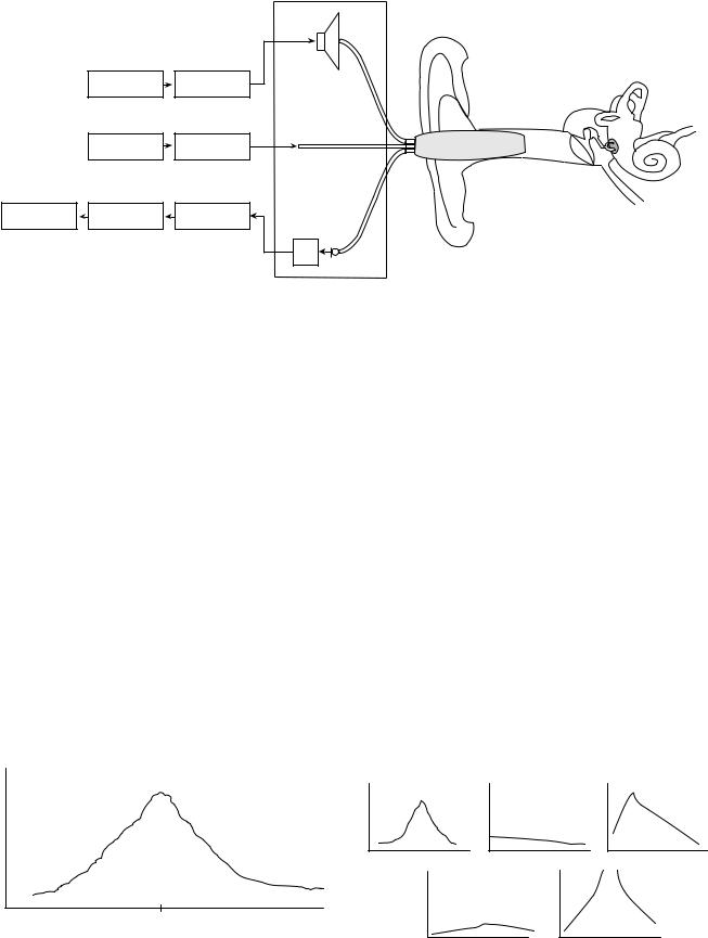
Many systems for recording auditory evoked potentials are now commercially available and are used widely. Components of the recording equipment typically include a stimulus generator capable of generating a variety of stimuli (e.g., clicks, tone bursts, tones), an attenuator, transducers for stimulus presentation (e.g., insert earphones, standard earphones, bone oscillator), surface electrodes, a differential amplifier, amplifier, filters, analog-to-digital converter, a signal averaging computer, data storage, display monitor, and printer. A simplified schematic diagram of a typical instrument is shown in Fig. 8.

In preparation for a typical single-channel recording, three electrodes are placed on the scalp. The electrodes often are called noninverting, inverting, and ground, but other terminology may be used (e.g., positive/negative or active/passive). A typical electrode montage is shown in Fig. 8, but electrode placements may vary depending on the potentials being recorded and the judgment of the clinician. Unwanted electrical or physiologic noise that may distort or obscure features of the response is reduced

Figure 8. Simple block diagram of an auditory evoked response audiometry system.

by the use of differential amplifiers with high common mode rejection ratios and filters. It is important to note that electrode placement, stimulus polarity, stimulus presentation rate, number of signal presentations, signal repetition rate, filter characteristics, stimulus characteristics, and sampling rate during analog-to-digital conversion all affect the recording, and so must be controlled by the clinician.

Classification of Evoked Auditory Potentials

After the onset of an auditory stimulus, neural activity in the form of a sequence of waveforms can be recorded. The amount of time between the onset of the stimulus and the occurrence of a designated peak or trough in the waveform is called the latency. The latency of some auditory evoked potentials can be as short as a few thousandths of a second, and other latencies can be 400 ms or longer. Auditory evoked potentials are often classified on the basis of their latencies. For example, a system of classification can divide the auditory evoked potentials into ‘‘early’’ [< 15 ms (e.g., electrocochleogram and auditory brainstem response)], ‘‘middle’’ [15–80 ms (e.g., Pa, Nb, and Pb)], and ‘‘late’’ [> 80 ms (e.g., P300)] categories. Various classification systems based on latencies have been described, and other forms of classification systems based on the neural sites presumed to be generating the potentials (e.g., brainstem, cortex) are also sometimes used.

It is important to note that recording most bioelectric potentials requires only passive cooperation from the patient, but for some electrical potentials originating in the cortex of the brain, patients must provide active, cognitive participation. In addition, certain potentials are affected by level of consciousness. These factors, combined with the purpose of the evaluation, are important in the selection of the waveforms to be recorded.

Auditory Threshold Estimation/Prediction with AEPs

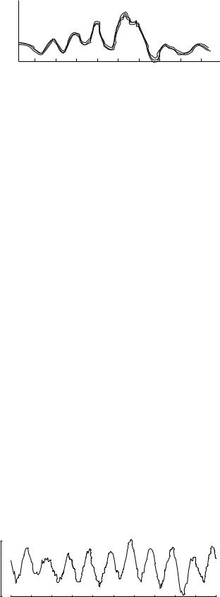
Auditory threshold estimations/predictions have been made on the basis of early, middle, and late potentials, but the evoked potentials most widely used for this purpose are those recorded within the first 10–15 ms after stimulus onset, particularly the so-called auditory brainstem response (ABR). An ABR evoked by a click consists of 5– 7 peaks that normally appear in this time frame (27–29). Typical responses are shown in Fig. 9. The figure depicts three complete ABRs, and each represents the algebraic average of 2048 responses to a train of acoustic transient stimuli. The ABR is said to be time-locked such that each of the prominent peaks occurs in the normal listener at

Amplitudein microvolts	III	IV
		V
	II
	I	VI	VI
			I

Time in milliseconds

Figure 9. Normal auditory brainstem response; three complete responses.

predictable time periods after stimulation. Reliability is a hallmark of the ABR, and helps assure the audiologist that a valid estimation of conduction time through auditory brainstem structures has been made. A brief, gated, square-wave signal (click) stimulus is often used to generate the response, and stimulus intensity is reduced until the amplitude of the most robust peak (Wave V) is indistinguishable from the baseline voltage.

The response amplitude and latency (which lengthens as stimulus intensity decreases) are used to estimate behavioral auditory thresholds. In some equipment arrangements, computer software is used to statistically analyze the potentials for threshold determination purposes. ABR thresholds obtained with click stimuli correlate highly with behavioral thresholds at 2000–4000 Hz when hearing sensitivity ranges from normal to the severe range hearing impairment. Click stimuli are commonly used in clinical situations because their transient characteristics can excite many neurons synchronously, and thus a large amplitude response is evoked. However, variability limits the usefulness of click-evoked thresholds for prediction/ estimation of auditory sensitivity of any particular patient (30), and the frequency specificity desired for audiometric purposes may not be obtained. As a result, gated tone bursts of differing frequencies are often used to estimate hearing sensitivity across the frequency range. These tonal stimuli can be embedded in bursts of noise to sharpen the frequency sensitivity and specificity of the test procedure.

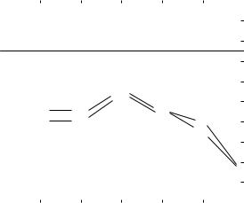
In recent years, another evoked potential technique similar to the ABR has been developed to improve frequency specificity in threshold estimation while maintaining good neural synchronization. This technique, the auditory steady-state response (ASSR), uses rapidly (amplitude or frequency) modulated pure tone carrier stimuli (see Fig. 10). Evidence suggests that the ASSR is particularly useful when hearing sensitivity is severely impaired because high intensity stimuli can be used

A

10 v

0

Modulation cycles

10

Figure 10. Auditory steady-state response.

AUDIOMETRY 99

(31). Research on the ASSR is ongoing, and this technique currently is considered to be a complement to click and tonal ABR in threshold estimation/prediction.

ACOUSTIC IMMITTANCE MEASUREMENT

Introduction

One procedure that helps audiologists interpret the results of conventional audiometry and other audiological tests is a measure of the ease with which energy can flow through the ear. Heaviside (1850–1925) coined the term impedance, as applied to electrical circuitry, and these principles were later applied in the United States during 1920s to acoustical systems (32). Mechanical impedance-measuring devices were initially designed for laboratory use, but electroacoustic measuring instruments were introduced for clinical use in the late 1950s (33). As acoustic impedance is difficult and expensive to measure accurately, measuring instruments using units of acoustic admittance are now widely used. The term used to describe measures incorporating the principles of both acoustic impedance and its reciprocal (acoustic admittance) is acoustic immittance. Modern instrumentation permits an estimate of ear canal and middle ear acoustic immittance (including resistive and reactive components).

Instrumentation

Commonly available immittance measuring devices (see Fig. 11) employ a probe-tone delivered to the tympanic membrane through the external ear canal. Sinusoids of differing frequencies are presented through a tube encased in a soft probe fitted snugly in the ear canal. The probe also contains a microphone and tubing connected to an air pump so that air pressure in the external ear canal can be varied from 400 to þ 400 mmH2O.

Immittance devices also typically have a signal generator and transducers that can be used to deliver high intensity tones at various frequencies for the purpose of acoustic reflex testing. The American National Standards Institute (ANSI) has published a standard (S3.39-1987) for immittance instruments (34).

Immittance Measurement Procedures

As mentioned earlier in this chapter, the middle ear transduces acoustic energy into mechanical form. The transfer function of the middle ear can be estimated by measuring acoustic immittance at the plane of the tympanic membrane. These measures are often considered (in conjunction with the results of other audiological tests) in determining the site of lesion of an auditory disorder.

Static Acoustic Immittance

The acoustic immittance of the middle ear system is usually estimated by subtracting the acoustic immittance of the ear canal. This value is termed the compensated static acoustic immittance and is measured in acoustic mhos (reciprocal of acoustic ohms). The peak compensated

100	AUDIOMETRY
				Probe tone
				speaker
		Probe tone	Amplifier
		oscillator	& control
		Air pump	Pressure valves	Probe
			& safety
	Processor &	A/D	Filter
	display screen	converter
				Pre
				amp Microphone

Figure 11. Block diagram of an acoustic immittance measuring device.

static acoustic immittance is obtained by adjusting the air pressure in the external ear canal so that a peak in the tympanogram exists. The magnitude of this peak, relative to the uncompensated immittance value, is clinically useful, because it can be compared with norms (e.g., 0.3 to 1.6 mmho) to determine the presence of middle ear pathology. It is important to note that at ear canal pressures of þ 200 daPa or more, the sound pressure level (SPL) in the ear canal is directly related to the volume of air in the external ear canal, because the contribution of the middle ear system is insignificant at that pressure. A measure of the external ear canal volume is a valuable measure that can be used to detect tympanic membrane perforations otherwise difficult to detect visually. That is, a large ear canal volume (i.e., a value considerably greater than 1.5 mL) indicates a measurement of both the external ear canal and the middle ear as a result of a perforation in the tympanic membrane.

Dynamic Acoustic Immittance (Tympanometry)

The sound pressure of the probe-tone directed at the eardrum is maintained at a constant level and the volume velocity is measured by the instrumentation while positive and negative air pressure changes are induced in the external ear canal.

Admittance (mmhos)

-400	0	+500
	Ear canal pressure (daPa)

Figure 12. Tympanogram of a normal ear.

The procedure is called tympanometry and the resulting changes in immittance are recorded graphically as a tympanogram. A typical tracing is seen in Fig. 12.

Admittance is at its maximum when the pressures on both sides of the tympanic membrane are equal. Sound transmission decreases when pressure in the ear canal is greater or less than the pressure at which maximum admittance occurs. As a result, in a normal ear, the shape of the tympanogram has a characteristic peaked shape (see Fig. 13) with the peak of admittance occurring at an air pressure of 0 decapascals (daPa).

Tympanograms are sometimes classified according to shape (Fig. 13) (35).

The Type A tympanogram shown in Fig. 13, so-called because of it’s resemblance to the letter ‘‘A’’, is seen in normal ears. When middle ear effusion is present, the fluid contributes to a decrease in admittance, regardless of the changes of pressure in the external ear canal. As a result, a characteristically flat or slightly rounded Type B tympanogram is typical. When the Eustachian tube malfunctions, the pressure in the middle ear can become negative relative to the air pressure in the external auditory canal. As energy flow through the ear is maximal when the pressure differential across the tympanic membrane is zero, tympanometry reveals maximum admittance when the pressure being

A

B

C

As

AD

Figure 13. Tympanogram types (see text for descriptions).

varied in the external ear canal matches the negative pressure in the middle ear. At that pressure, the peak admittance will be normal but will occur at an abnormal negative pressure value. This tympanogram type is termed a Type C. It is important to note that variations exist of the type A tympanogram associated with specific pathophysiology affecting the middle ear. For example, if the middle ear is unusually stiffened by ear disease, the height of the peak may be reduced (Type As). Similarly, if middle ear pathology such as a break in the ossicular chain occurs, the energy flow may be enhanced, which is reflected in the Type Ad tympanogram depicted in Fig. 13.

Multifrequency Tympanometry

Under certain circumstances, particularly during middle ear testing of newborns and in certain stages of effusion in the middle ear, responses to the 226 Hz probe-tone typically used in tympanometry may fail to reveal immittance changes caused by disorders of the middle ear. In these circumstances, tympanometry with probe-tone frequencies above 226 Hz may be very useful in the detection of middle ear dysfunction. With probe-tone frequencies above 226 Hz, tympanometric shapes are more complex. More specifically, multifrequency tympanometric tracings normally progress through an expected sequence of shapes as probe frequency increases (36), and deviations from the expected progression are associated with certain pathologies.

Acoustic Reflex Measurement

In humans, a sufficiently intense sound causes a reflexive contraction of the middle ear muscles in both ears, acoustically stiffening the middle ear systems in each ear, called the acoustic reflex and is a useful tool in the audiometric test battery. When the reflex occurs, energy flow through both middle ears is reduced, and the resulting change in immittance can be detected in the probe ear by an immittance measuring device. Intense tones can be introduced to the probe ear (ipsilateral stimulation) or by earphone to the ear opposite the probe ear (contralateral stimulation).

One acoustic reflex measure is the minimum sound intensity necessary to elicit the reflex. The minimum sound pressure level necessary to elicit the reflex is called the acoustic reflex threshold. Acoustic reflex thresholds that are from 70 to 100 dBHL are generally considered to be in the normal range when pure tone stimuli are used. In general, the acoustic reflex thresholds in response to broadband noise stimuli tend to be lower than those for pure tones. Reduced or elevated thresholds, as well as unusual acoustic reflex patterns, are used by audiologists to localize the site of lesion and as one method of predicting auditory sensitivity.

OTOACOUSTIC EMISSIONS

When sound is introduced to the ear, the ear not only is stimulated by sound, it can also generate sounds that can be detected in the ear canal. The generated sounds, so-

AUDIOMETRY 101

called otoacoustic emissions, have become the basis for the development of another tool that audiologists can use to assess the auditory system. In the following section, otoacoustic emissions will be described, and their relationship to conventional audiometry will be discussed.

Otoacoustic Emissions—Historical Perspective

Until relatively recently, the cochlea was viewed as a structure that converted mechanical energy from the middle ear into neural impulses that could be transmitted to and used by the auditory nervous system. This conceptual role of the cochlea was supported by the work on human cadavers of Georg von Bekesy during the early and middle 1900s, and summarized in 1960 (37). In Nobel Prizewinning research, von Bekesy developed theories to account for the auditory system’s remarkable frequency sensitivity, and his views were widely accepted. However, a different view of the cochlea was proposed by one of von Bekesy’s contemporaries, Thomas Gold, who suggested that processing in the cochlea includes an active process, a mechanical resonator (38). This view, although useful in explaining cochlear frequency selectivity, was not widely embraced at the time it was proposed.

In later years, evidence in support of Gold’s idea of active processing in the cochlea accumulated. Particularly significant were direct observations of outer hair cell motility (39). In addition, observed differences in inner hair cell and outer hair cell innervation such as direct efferent innervation of outer but not inner hair cells (40) suggested functional differences in the two cell types. Most relevant to the present discussion were reports of the sounds that were recorded in the ear canal (41) and attributed to a mechanical process occurring in the cochlea, which are now known as otoacoustic emissions.

Otoacoustic Emissions—Description

Initially, otoacoustic emissions (OAEs) were thought to originate from a single mechanism, and emissions were classified on the basis of the stimulus conditions under which they were observed. For example, spontaneous otoacoustic emissions (SOAEs) are sounds that occur spontaneously without stimulation of the hearing mechanism. Two categories of otoacoustic emissions that are most widely used clinically by audiologists are (1) transient otoacoustic emissions (TOAEs), which are elicited by a brief stimulus such as an acoustic click or a tone burst, and (2) distortion product otoacoustic emissions (DPOAEs), which are elicited by two tones (called primaries) that are similar, but not identical, in frequency. A third category of otoacoustic emissions that may prove helpful to audiologists in the future is the stimulus frequency otoacoustic emission (SFOAE), which is elicited with a pure tone. Currently, SFOAEs are used by researchers studying cochlear function, but they are not used widely in clinical settings.

Recent research indicates that, contrary to initial thinking, otoacoustic emissions are generated by at least two mechanisms, and a separate classification system has been proposed to reflect improved understanding of the physical basis of the emissions. Specifically, it is believed that the

102 AUDIOMETRY

mechanisms that give rise to evoked otoacoustic emissions include (1) a nonlinear distortion source mechanism and (2) a reflection source that involves energy reflected from irregularities within the cochlea such as variations in the number of outer hair cell motor proteins or spatial variations in the number and geometry of hair cell distribution (42). Emissions currently recorded in the ear canal for clinical purposes are thought to be mixtures of sounds generated by these two mechanisms.

Instrumentation

Improved understanding of the mechanisms that generate otoacoustic emissions may lead to new instrumentation that can ‘‘unmix’’ evoked emissions. Currently, commercially available clinical equipment records ‘‘mixed’’ emissions and includes a probe placed in the external ear canal that both delivers stimuli (i.e., pairs of primary tonal stimuli across a broad range of frequencies, clicks or tone-bursts) and records resulting acoustic signals in the ear canal. The microphone in the probe equipment is used in (1) the verification of probe fit, (2) monitoring probe status (e.g., for cerumen occlusion), (3) measuring noise levels, (4) verifying stimulus characteristics, and (5) detecting emissions. Otoacoustic measurement recording entails use of probe tips of various sizes to seal the probe in the external ear canal and hardware/software that control stimulus parameters and protocols for stimulus presentation. The computer equipment performs averaging of responses time-locked to stimulus presentation, noise measurement, artifact rejection, data storage, and so on, and can provide stored normative data and generate printable reports. An example of a typical DPOAE data display is shown in Fig. 14.

It is important to note that outer or middle ear pathology can interfere with transmission of emissions from the cochlea to the ear canal, and thus the external ear canal and middle ear status are important factors in data interpretation. Also, although otoacoustic emissions ordinarily are not difficult to record and interpret, uncooperative

	30.0
	20.0
		x
	10.0
SPL	x	x	x	x	x
	0.0				x
dB
	–10.0
	–20.0
	–30.0
	1K	2K		4K	8K	16K

Frequency (Hz)

Figure 14. DPAOE responses from 1000 to 6,000 Hz from the left ear of a normal listener. X ¼ DPOAE response amplitudes; squares ¼ physiologic noise floor; bold curves ¼ 95% confidence limits for normal ears.

patient behavior and high noise levels can hamper or even preclude measurement of accurate responses.

Otoacoustic Emissions—Clinical Applications

Measurement of otoacoustic emissions is used routinely as a test battery component of audiometric evaluations in children and adults, and it is particularly useful for monitoring cochlear function (e.g., in cases of noise exposure and during exposure to ototoxic medication) as well as differentiating cochlear from neural pathology. Currently, otoacoustic emission evaluation is also useful, either alone or in combination with evoked potential recording, in newborn hearing screening. In addition, OAE assessment is sometimes used in preschool and school-age hearing screening, as well as with patients who may be unwilling to cooperate during audiometry.

Otoacoustic Emissions and Audiometric Threshold

Prediction/Estimation

Audiologists do not use otoacoustic emissions as a measure of ‘‘hearing’’ because OAEs constitute an index of cell activity in the inner ear, not ‘‘hearing.’’ Research suggests, however, that otoacoustic emissions may become an important indicator for predicting/estimating auditory thresholds when conventional audiometry cannot be conducted (42).

Many sources of variability exist that affect DPOAE use in audiometric threshold prediction/estimation, including variability with respect to etiology of the hearing loss, age, gender, and uncertainty regarding locations of DPOAE generation and their relationship to audiometric test frequencies. Individual DPOAE amplitude variation, intraand inter-subject variations occurring at different frequencies and at different stimulus levels, and the mixing of emissions from at least two different regions of the cochlea (as described above) can reduce frequency selectivity and specificity in DPOAE measurement.

It has been suggested that developing methods to ‘‘unmix’’ the emissions associated with different generators (e.g., through the use of suppressor tones to reduce or eliminate one source component or with the use of Fourier analysis to analyze the emissions) may reduce variability and improve specificity in threshold prediction/estimation and determination of etiology (41). It is likely that future commercial otoacoustic measurement instruments will enable the user to differentiate distortion source emissions from reflection source emissions and that this improvement will lead to more widespread use of otoacoustic emissions in audiometric threshold estimation and prediction.

BIBLIOGRAPHY

1.American Academy of Audiology. Scope of practice. Audiol Today 2004;15(3):44–45.

2.American National Standards Institute. Methods of manual pure tone threshold audiometry. (ANSI S3.21-2004). New York: ANSI; 2004.

3.Bergman M. On the origins of audiology: American wartime military audiology. Audiol Today Monogr 2002;1:1–28.

4.Seashore CE. An Audiometer. University of Iowa Studies in Psychology (No. 2). Iowa City, NA: University of Iowa Press; 1899.

5.Bunch CC. Clinical Audiometry. St. Louis, MO: C. V. Mosby; 1943.

6.Fowler EP, Wegel RL. Presentation of a new instrument for determining the amount and character of auditory sensation. Trans Am Otol Soc 1922;16:105–123.

7.Bunch CC. The development of the audiometer. Laryngoscope 1941;51:1100–1118.

8.Carhart R. Clinical application of bone conduction audiometry. Archi Otolaryngol 1950;51:798–808.

9.American National Standards Institute. Specification of audiometers. (ANSI-S3.6-1996). New York: ANSI; 1996.

10.American National Standards Institute. Maximum permissible ambient noise levels for audiometric test rooms. (ANSI- S3.1-1999 [R2003]). New York: ANSI; 1999.

11.Breakwell GM, Hammond S, Fife-Shaw C. Research Methods in Psychology. 2nd ed. London: Sage; 2000. p 200–205.

12.von Bekesy G. A new audiometer. Acta Oto-laryngologica Stockholm 1947;35:411–422.

13.Jerger J. Bekesy audiometry in analysis of auditory disorders. J Speech Hear Res 1960;3:275–287.

14.Jerger J, Herer G. Unexpected dividend in Bekesy audiometry. J Speech Hear Disord 1961;26:390–391.

15.Jerger S, Jerger J. Diagnostic value of Bekesy comfort loudness tracings. Arch Otolaryngol 1974;99:351–360.

16.Carhart R, Jerger J. Preferred method for clinical determination of pure-tone thresholds. J Speech Hear Disord 1959;24: 330– 345.

17.Feldmann H. A history of audiology: A comprehensive report and bibliography from the earliest beginnings to the present. Translations Beltone Institute Hear Res 1960;22:1–111. [Translated by Tonndorf J. from Die Geschichtliche Entwicklung der Horprufungsmethoden, Kuze Darstellung and Bibliographie von der Anfrongen bis zur Gegenwart. In: Leifher H, Mittermaiser R, Theissing G, editors. Zwanglose Abhandunger aus dem Gebeit der Hals-Nasen-Ohren-Heilkunde. Stuttgart: Georg Thieme Verlag; 1960.]

18.Hudgins CV, Hawkins, JE Jr, Karlin JE, Stevens SS. The development of recorded auditory tests for measuring hearing loss for speech. Laryngoscope 1947;57:57–89.

19.Olsen WO, Matkin ND. Speech audiometry. In: Rintelmann WF, editor. Hearing Assessment. 2nd ed. Austin, TX: Pro-Ed; 1991. 39–140.

20.Fletcher H. Speech and Hearing. Princeton NJ: Von Nostrand; 1929.

21.Fletcher H. A method of calculating hearing loss for speech from an audiogram. Acta Otolaryngologica 1950; (Suppl 90): 26–37.

22.Carhart R. Observations on the relations between thresholds for pure tones and for speech. J Speech Hear Disord 1971; 36:476–483.

23.Beattie RC, Edgerton BJ, Svihovec DV. An investigation of Auditec of St. Louis recordings of Central Institute for the Deaf spondees. J the Am Audiol Soc 1975;1:97–101.

24.Cambron NK, Wilson RH, Shanks JE. Sondaic word detection and recognition functions for female and male speakers. Ear Hear 1991;12:64–70.

AUDIOMETRY 103

25.Loomis A, Harvey E, Hobart G. Disturbances of patterns in sleep. J Neurophysiol 1938;1:413–430.

26.Clark WA Jr, Goldstein MH Jr, Brown RM, Molnar CE, O’Brien DF, Zieman HE. The average response computer (ARC): A digital device for computing agerages and amplitudes and time histograms of physiological responses. Trans of IRE 1961;8:46–51.

27.Jewett DL, Romano MN, Williston JS. Human auditory evoked potentials: Possible brainstem components detected on the scalp. Science 1970;167:1517–1518.

28.Jewett DL, Williston JS. Auditory evoked far fields averaged from the scalp of humans. Brain 1971;94:681–696.

29.Stapells DR, Oates P. Estimation of the pure-tone audiogram by the auditory brainstem response: A review. Audiol Neurootol 1997;3(5):257–280.

30.Rance G, Briggs RJS. Assessment of hearing in infants with moderate to profound impairment: The Melbourne experience with auditory stead-state evoked potential testing. Ann Otol Rhinol Laryngol 2002;111(5) (Part 2, Suppl. 189):22–28.

31.Swanepoel D, Roode R. Auditory steady-state responses for children with severe to profound hearing loss. Arch of Otolaryngol Head Neck Surg 2004;130(5):531–535.

32.Margolis RH, Hunter LH. Acoustic Immittance Measurements. In: Roeser RJ, Valente M, Hosford-Dunn H, editors. Audiology Diagnosis. New York: Thieme; 2002. pp 381–423.

33.Terkildsen K, Nielsen S. An electroacoustic impedance measuring bridge for clinical use. Arch Otolaryngol 1960;72:339–346.

34.American National Standards Institute. National Standard Specifications for instruments to measure aural acoustic impedance and admittance. (ANSI S3.39-1987). New York: ANSI; 1987.

35.Jerger J. Clinical experience with impedance audiometry. Arch Otolaryngol 1970;92:311–324.

36.Vanhuyse VJ, Creten WL, Van Camp KJ. On the W-notching of tympanograms. Scand Audiol 1975;4:45–50.

37.von Bekesy G. Experiments in Hearing. New York: McGraw Hill; 1960.

38.Gold T. Hearing. II. The physical basis of the acton of the cochlea. Proc Roy Soc Brit 1948;135:492–498.

39.Brownell WE, Bader CR, Bertrand D, Ribaupierre Y. Evoked mechanical responses of isolated cochlear outer hair cells. Science 1985;227:194–196.

40.Smith CA. Innervation pattern of the cochlea. Ann Otol Rhinol Otolaryngol 1961;70:504–527.

41.Kemp DT. Stimulated acoustic emissions from within the human auditory system. J Acoust Soc Am 1978;64:1386–1391.

42.Shera CA. Mechanisms of mammalian otoacoustic emission and their implications for the clinical utility of otoacoustic emissions. Ear Hear 2004;25:86–97.

See also COCHLEAR PROSTHESES; COMMUNICATION DEVICES.

AUDITORY IMPLANTS. See COCHLEAR

PROSTHESES.

AUGMENTATIVE COMMUNICATION

SYSTEM. See COMMUNICATION DEVICES.