Intermediate Physics for Medicine and Biology - Russell K. Hobbie & Bradley J. Roth

21. Mechanics

a)

b)

c)

d)

e)

100 m

FIGURE 1.1. Objects ranging in size from 1 mm down to 1 µm. (a) A paramecium, (b) an alveolus (air sac in the lung),

(c) a cardiac cell, (d) red blood cells, and (e) Escherichia coli bacteria.

250 µm long [Fig. 1.1(a)]. The cells in multicellular animals tend to be somewhat smaller than protozoans. For instance, the mammalian cardiac cell (a muscle cell found in the heart, Chapter 7) shown in Fig. 1.1(c) is about 100 µm long and 20 µm in diameter. Nerve cells have a long fiber-like extension called an axon. Axons come in a variety of sizes, from 1 µm diameter up to tens of microns. The squid contains a giant axon nearly one millimeter in diameter. This axon played an important role in our understanding of how nerves work (Chapter 6).

Our red blood cells (erythrocytes) carry oxygen to all parts of our body. (Actually, red blood cells are not true cells at all, but rather “corpuscles”). Red blood cells are disk-shaped, with a diameter of about 8 µm and a thickness of 2 µm [Fig. 1.1(d)]. Blood flows through a branching network of vessels (Section 1.17), the smallest of which are capillaries. Each capillary has a diameter of about 8 µm, meaning that the red blood cells can barely pass through it single-file.

One valuable skill in physics is the ability to make order-of-magnitude estimates, meaning to calculate something approximately right. For instance, suppose we want to calculate the number of cells in the body. This is a di cult calculation, because cells come in all sizes and shapes. But for some purposes we only need an approximate answer (say, within a factor of ten). For example: cells are roughly 10 µm in size, so their volume is about (10 µm)3, or (10×10−6)3 = 10−15 m3. An adult is roughly 2 m tall and about 0.3 m wide, so our volume is about 2 m × 0.3 m × 0.3 m, or 0.18 m3. We are made up almost entirely of cells, so the number of cells in our body is about0.18 m3 / 10−15 m3 , or roughly 2 × 1014. Some problems at the end of the chapter ask you to make similar order-of-magnitude calculations.

a)	b)
	c)
	d)
	e)
	100 nm

FIGURE 1.2. Objects ranging in size from 1 µm down to 1 nm.

(a) the human immunodeficiency virus (HIV), (b) hemoglobin molecules, (c) a cell membrane, (d) a DNA molecule, (e) glucose molecules.

Most cells are larger than a few microns. But many cells (called eukaryotes) are complex structures that contain organelles about this size. Mitochondria, organelles where many of the chemical processes providing cells with energy take place, are typically about 2 µm long. Protoplasts, organelles found in plant cells where photosynthesis changes light energy to chemical energy, are also about 2 µm long.

The simplest cells are called prokaryotes and contain no subcellular structures. Bacteria are the most common prokaryotic cells. The bacterium Escherichia coli, or E. coli, is about 2 µm long [Fig. 1.1(e)], and has been studied extensively.

To examine structures smaller than bacteria, we must measure lengths that are smaller than a micron. Onethousandth of a micron is called a nanometer (1 nm = 10−9 m). Figure 1.2 shows objects having lengths from 1 nm to 1 µm. E. coli bacteria, which seemed so tiny compared to cells in Fig. 1.1, are giants on the nanometer length scale, being 20 times longer than the 100 nm scale bar in Fig. 1.2. Viruses are tiny packets of genetic material encased in protein. On their own they are incapable of metabolism or reproduction, so some scientist don’t even consider them as living organisms. Yet, they can infect a cell and take control of its metabolic and reproductive functions. The length scale of viruses is one-tenth of a micron, or 100 nm. For instance, HIV (the virus that causes AIDS) is roughly spherical with a diameter of about 120 nm [Fig. 1.2(a)]. Some viruses, called bacteriophages, infect and destroy bacteria. Most viruses are too small to see in a light microscope. The resolution of a microscope is limited by the wavelength of light, which is about 500 nm (Chapter 14). Thus, with a microscope we can study cells in detail, we can see bacteria without much resolution, and we can barely see viruses, if we can see them at all.

Below 100 nm, we enter the world of individual molecules. Proteins are large, complex macromolecules that are vitally important for life. For example, hemoglobin is

the protein in red blood cells that binds to and carries oxygen. Hemoglobin is roughly spherical, about 6 nm in diameter [Fig. 1.2(b)]. Many biological functions occur in the cell membrane (see Chapter 5). Membranes are made up of layers of lipid (fat), often with proteins and other molecules embedded in them [Fig. 1.2(c)]. A typical cell membrane is about 10 nm thick. The molecule adenosine triphosphate (ATP), crucial for energy production and distribution in cells, is about 2 nm long (Chapter 3). Chemical energy is stored in molecules called carbohydrates. A common (and relatively small) carbohydrate is glucose (C6H12O6), which is about 1 nm long [Fig. 1.2(e)]. Genetic information is stored in long, helical strands of deoxyribonucleic acid (DNA). DNA is about 2.5 nm wide, and the helix completes a turn every 3.4 nm along its length [Fig. 1.2(d)].

At the 1-nm scale and below, we reach the world of small molecules and individual atoms. Water is the most common molecule in our body. It consists of two atoms of hydrogen and one of oxygen. The distance between adjacent atoms in water is about 0.1 nm. The distance 0.1 nm (100 pm) is used so much at atomic length scales that

˚

it has earned a nickname: the angstrom (A). Like the cm, this unit is going out of fashion as the use of nanometer becomes more common. Individual atoms have diameters of 100 or 200 pm.

Below the level of 100 pm, we leave the realm of biology and enter the world of subatomic physics. The nuclei of atoms (Chapter 17) are very small, and their sizes are measured in femtometers (1 fm = 10−15 m).

One cannot possibly memorize the size of all biological objects: there are simply too many. The best one can do is remember a few mileposts along the way. Table 1.2 contains a rough guide to how large a few important biological objects are. Think of these as rules of thumb. Given the diversity of life, one can certainly find exceptions to these rules, but if you memorize Table 1.2 you will have a rough framework to organize your thinking about size. To examine the relative sizes of objects in more detail, see Morrison et al. (1994) or Goodsell (1998).

1.2 Forces and Translational Equilibrium

3

TABLE 1.2. Approximate sizes of biological objects.

Object	Size
Protozoa	100 µm
Cells	10 µm
Bacteria	1 µm
Viruses	100 nm
Macromolecules	10 nm
Molecules	1 nm
Atoms	100 pm

One finds experimentally that an object is in translational equilibrium if the vector sum of all the forces acting on the body is zero. Equilibrium means that the object either remains at rest or continues to move with a constant velocity. That is, it is not accelerated. Translational means that only changes of position are being considered; changes of orientation of the object with respect to the axes are ignored.

We must consider all the forces that act on the object. If the object is a person standing on both feet, the forces are the upward force of the floor on each foot and the downward force of gravity on the person (more accurately, the vector sum of the gravitational force on every cell in the person). We do not consider the downward force that the person’s feet exert on the floor. It is also possible to replace the sum of the gravitational force on each cell of the body with a single downward gravitational force acting at one point, the center of gravity of the body.

The forces that add to zero to give translational equilibrium need not all act at one point on the object. If the object is a person’s leg and the leg is at rest, there are three forces exerted on the leg by other objects (Fig. 1.3). Force F1 is the push of the floor up on the bottom of the foot. The various pushes and pulls of the rest of the body

1.2Forces and Translational Equilibrium

There are several ways that we can introduce the idea of force, depending on the problem at hand and our philosophical bent. For our present purposes it will su ce to say that a force is a push or a pull, that forces have both a magnitude and a direction, and that they give rise to accelerations through Newton’s second law, F = ma. Experiments show that forces add like displacements, so they can be represented by vectors. (Some of the properties of vectors are reviewed in Appendix B; others are introduced as needed.) Vectors will be denoted by boldfaced characters.

FIGURE 1.3. Forces on the leg in equilibrium. Each force is exerted by some other object. (a) The points of application are widely separated. (b) The sum of the forces is zero.

41. Mechanics

on the leg through the hip joint and surrounding muscles have been added together to give F2. The gravitational pull of the earth downward on the leg is F3. Force F1 acts on the bottom of the leg, F2 acts on the top, and F3 acts somewhere in between. If the leg is in equilibrium the sum of these forces is zero, as shown in Fig. 1.3(b). Although the points of application of the forces can be ignored in considering translational equilibrium, they are important in determining whether or not the object is in rotational equilibrium. This is discussed shortly.

The Greek letter Σ (capital sigma) is usually used to mean a sum of things. With this notation, the condition for translational equilibrium can be written

Fi = 0.

(1.1)

i

The subscript i is used to label the di erent forces acting on the body. A notation this compact has a lot hidden in it. This is a vector equation, standing for three equations:

Fix = 0,

i

Fiy = 0,

(1.2)

i

Fiz = 0.

i

Often the subscript i is omitted and the equations are

written as Fx = 0, Fy = 0, Fz = 0. In this notation, a component is positive if it points along the positive axis and negative if it points the other way.

Sometimes, as in the next example, we draw forces in particular directions and assume that these directions are positive. If the subsequent algebra happens to give a solution that is negative, the force points opposite the direction assumed.

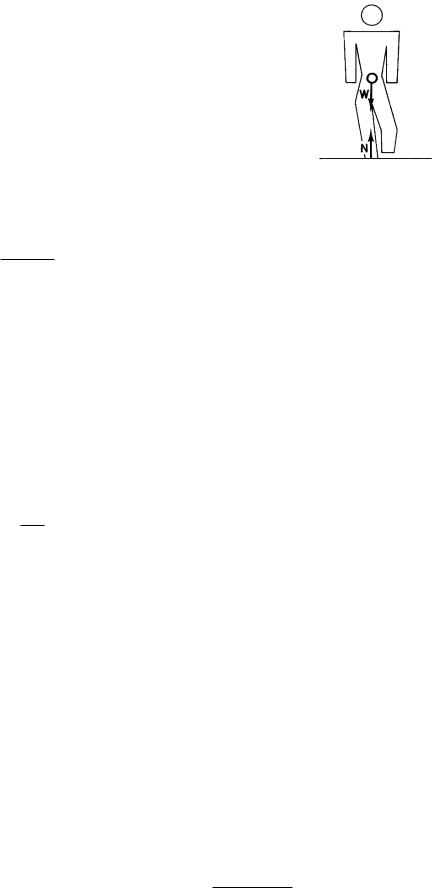
As an example, consider the person standing on both feet as in Fig. 1.4. The earth pulls down at some point with force W. The floor pushes up on the right foot with force F1 and on the left foot with force F2. To determine what the condition for translational equilibrium tells us

about the forces, draw the force diagram or free-body diagram of Fig. 1.4(b). This diagram is an abstraction that ignores the points at which the forces are applied to the body. We can get away with this abstraction because we are considering only translation. When we consider rotational equilibrium, we will have to redraw the diagram showing the points at which the various forces act on the person. If all the forces are vertical, then there is only one component of each force to worry about, and the equilibrium condition gives F1 + F2 − W = 0, or F1 + F2 = W . The total force of the floor pushing up on both feet is equal to the pull of the earth down.

If there is a sideways force on each foot, translational equilibrium provides two conditions: F1x + F2x = 0, and F1y + F2y − W = 0.

This is all that can be learned from the condition for translational equilibrium. If the person stands on one foot, then F1 = 0 and F2 = W . If the person stands with equal force on each foot, then F1 = F2 = W/2.

1.3 Rotational Equilibrium

If the object is in rotational equilibrium, then another condition must be placed upon the forces. Rotational equilibrium means that the object either does not rotate or continues to rotate at a constant rate (with a constant number of rotations per second). Consider the object of Fig. 1.5, which is a rigid rod pivoted at point X so that it can rotate in the plane of the paper. Forces F1 and F2 are applied to the rod in the plane of the paper at distances r1 and r2 from the pivot and perpendicular to the rod. The pivot exerts the force F3 on the rod needed to maintain translational equilibrium. If both F1 and F2 are perpendicular to the rod, they are parallel. They must also be parallel to F3, and translational equilibrium requires that

F3 = F1 + F2.

Experiment shows that there is no rotation of the rod if F1r1 = F2r2. The condition for rotational equilibrium can be stated in a form analogous to that for translational

equilibrium if we define the torque, τ , to be
τi = riFi.	(1.3)

With this definition goes an algebraic sign convention: the torque is positive if it tends to produce a counterclockwise rotation. The rod is in rotational equilibrium if

	FIGURE 1.4. A person standing. (a) The forces on the person.	FIGURE 1.5. A rigid rod free to rotate about a pivot at point
	(b) A free-body or force diagram.
		X.

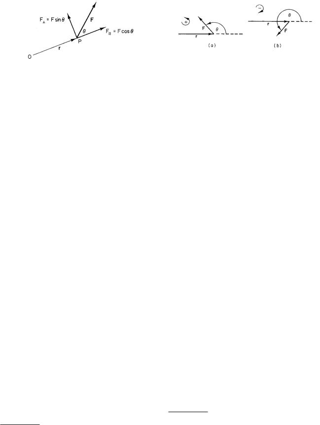
FIGURE 1.6. A force F is applied to an object at point P . The object can rotate about point O. Vectors r and F determine the plane of the paper.

the algebraic sum of all the torques is zero:

τi =	riFi = 0.	(1.4)
i	i

Note that F3 contributes nothing to the torque because r3 is zero.

The torque is defined about a certain point, X. It depends on the distance from the point of application of each force to X.2 As long as the object is in translational equilibrium, the torque can be evaluated around any point. This theorem, which we will not prove, often allows calculations to be simplified, because taking torques about certain points can cause some forces not to contribute to the torque equation.

The torque can also be calculated if the force is not at right angles to the rod. Imagine an object free to rotate about point O in Fig. 1.6. Force F lies in the plane of the paper but is applied in some arbitrary direction at point P . The vectors r and F determine the plane of the paper if they are not parallel. Force F can be resolved into two components: one parallel to r, F = F cos θ, and the other perpendicular to r, F = F sin θ. The component parallel to r will not cause any rotation about point O. (Pull on an open door parallel to the plane of the door; there is

no rotation.) The torque is therefore
τ = rF = rF sin θ.	(1.5)

The perpendicular distance from the line along which the force acts to point X is r sin θ. It is often called the moment arm, and the torque is the magnitude of the force multiplied by the moment arm.

The angle θ is the angle of rotation from the direction of r to the direction of F. It is called positive if the rotation is counterclockwise. For the angle shown in Fig. 1.6 sin θ has a positive value, and the torque is positive. Figure 1.7(a) shows an angle between 90 ◦ and 180 ◦ for which the torque and sin θ are still positive. Figure 1.7(b) shows an angle between 180 ◦ and 360 ◦, for which both

2The discussion associated with Fig. 1.5 suggests that torque is taken about an axis, rather than a point. In a three-dimensional problem the torque is taken about a point.

1.4 Vector Product

5

FIGURE 1.7. (a) When θ is between 0 ◦ and 180 ◦, both sin θ and the torque are positive. (b) When θ is between 180 ◦ and 360 ◦, both sin θ and the torque are negative.

the torque and sin θ are negative. In all cases, Eq. 1.5 gives the correct sign for the torque.

To summarize: the torque due to force F applied to a body at point P must be calculated about some point O. If r is the vector from O to P , the magnitude of the torque is equal to the magnitude of r times the magnitude of F, times the sine of the angle between r and F. The angle is measured counterclockwise from r to F.

1.4 Vector Product

Torque can be thought of as a vector, τ . Its magnitude is F r sin θ. The only direction uniquely defined by vectors r and F is perpendicular to the plane in which they lie. This is also the direction of an axis about which the torque would cause a rotation. However, there is ambiguity about which direction along this line to assign to the torque. The convention is to say that a positive torque points in the direction of the thumb of the right hand when the fingers curl in the direction of positive rotation from r to F.3 When r and F point in the same direction, so that no plane is defined, the magnitude of the torque is zero.

The product of two vectors according to the foregoing rules is called the cross product or vector product of the two vectors. One can use a shorthand notation

τ = r × F.

(1.6)

There is another way to write the cross product. If both r and F are resolved into components, as shown in Fig. 1.8, then the cross product can be calculated by applying the rules above to the components. Since Fy is perpendicular to rx and parallel to ry , its only contribution is a counterclockwise torque rxFy . The only contribution from Fx is a clockwise torque, −ry Fx. The magnitude of the cross product is therefore

τ = rxFy − ry Fx.

(1.7)

3This arbitrariness in assigning the sense of τ means that it does not have quite all the properties that vectors usually have. It is called an axial vector or a pseudovector. It will not be necessary in this book to worry about the di erence between a real vector and an axial vector.

61. Mechanics

FIGURE 1.8. The cross product r ×F is calculated by resolving r and F into components.

Note that this is the (signed) sum of each component of the force multiplied by its moment arm.

The equivalence of this result to Eq. 1.5 can be verified by writing Eq. 1.7 as

τ = (r cos β)(F sin α) − (r sin β)(F cos α),

τ = rF (sin α cos β − cos α sin β) .

There is a trigonometric identity that

sin (α − β) = sin α cos β − cos α sin β.

Since θ = α − β (from Fig. 1.8), this is equivalent to τ = rF sin θ.

When vectors r and F lie in the xy plane, τ points along the z axis. If r and F point in arbitrary directions, Eq. 1.7 gives the z component of τ . One can apply the same reasoning for other components and show that

τx = ry Fz − rz Fy ,
τy = rz Fx − rxFz ,	(1.8)
τz = rxFy − ry Fx.

If you are familiar with the rules for evaluating determinants, you will see that this is equivalent to the notation

FIGURE 1.9. Simplified anatomy of the foot.

this tendon on the calcaneus when a person is standing on the ball of one foot, assume that the entire foot can be regarded as a rigid body. This is our first example of creating a model of the actual situation. We try to simplify the real situation to make the calculation possible while keeping the features that are important to what is happening. In this model the internal forces within the foot are being ignored.

Figure 1.10 shows the force exerted by the tendon on the foot (FT ), the force of the leg bones (tibia and fibula) on the foot (FB ), and the force of the floor upward, which is equal to the weight of the body (W). The weight of the foot is small compared to these forces and will be neglected. Measurements on a few people suggest that

the angle the Achilles tendon makes with the vertical is about 7 ◦.

Translational equilibrium requires that
FT cos(7 ◦) + W − FB cos θ = 0,	(1.10)
FT sin(7 ◦) − FB sin θ = 0.

FT

		xˆ		yˆ		ˆz
τ =
		r	x	r	y	r	z	.
		F	x	F	y	F	z

(1.9)	7¡	W
	rT	r W
	5.6 cm	10 cm

1.5 Force in the Achilles Tendon

The equilibrium conditions can be used to understand many problems in clinical orthopedics. Two are discussed in this book: forces that sometimes cause the Achilles tendon at the back of the heel to break, and forces in the hip joint.

The Achilles tendon connects the calf muscles (the gastrocnemius and the soleus) to the calcaneus at the back of the heel (Fig. 1.9). To calculate the force exerted by

FB θ

FIGURE 1.10. Forces on the foot, neglecting its own weight.

To write the condition for rotational equilibrium, we need to know the lengths of the appropriate vectors rT and rW , assuming that the torques are taken about the point where FB is applied to the foot. In our simple model we ignore the contributions of the horizontal components of any forces to the torque equation. This is not essential (if we are willing to make more detailed measurements), but it simplifies the equations and thereby makes the process clearer. The horizontal distances measured on one of the authors are rT = 5.6 cm and rW = 10 cm, as shown in Fig. 1.10. The torque equation is

10W − 5.6FT cos 7 ◦ = 0.

(1.11)

This equation can be solved for the tension in the tendon:

FT =	10W	= 1.8W.	(1.12)
	5.6 cos 7 ◦

This result can now be used in Eq. 1.10 to find FBy = FB cos θ:

(1.8)(W )(0.993) + W = FB cos θ,
2.8W = FB cos θ.	(1.13)
From Eqs. 1.10 and 1.12, we get
(1.8)(W )(0.122) = FB sin θ,
0.22W = FB sin θ.	(1.14)

Equations 1.13 and 1.14 are squared and summed and the square root taken to give FB = 2.8W , while they can be divided to give

tan θ = 0.22 = 0.079, 2.8

θ = 4.5 ◦ .

The tension in the Achilles tendon is nearly twice the person’s weight, while the force exerted on the leg by the talus is nearly three times the body weight. One can understand why the tendon might rupture.

1.6 Forces on the Hip

The forces in the hip joint can be several times the person’s weight, and the use of a cane can be very e ective in reducing them.

As a person walks, there are moments when only one foot is on the ground. There are then two forces acting on the body as a whole: the downward pull of the earth W and the upward push of the ground on the foot N . The pull of the earth may be regarded as acting at the center of gravity of the body [Halliday et al. (1992, Chap. 13)]. The center of gravity is located on the midline (if the limbs are placed symmetrically), usually in the lower abdomen [Williams and Lissner (1962), Chap. 5.] If torques are taken about the foot, then the center of gravity must

1.6 Forces on the Hip

7

FIGURE 1.11. A person standing on one foot must place the foot under the center of gravity, which is on or near the midline.

be directly over the foot so that there will be no torque from either force. This situation is shown in Fig. 1.11. The condition for translational equilibrium requires that

N = W .

The anatomy of the pelvis, hips, and leg is shown schematically in Fig. 1.12. Fourteen muscles and several ligaments connect the pelvis to the femur. Extensive measurements of the forces exerted by the abductor4 muscles in the hip have been made by Inman (1947). If the leg is considered an isolated system as in Fig. 1.12, the following forces act:

F: The net force of the abductor muscles, acting on the greater trochanter. These muscles are primarily the gluteus medius and gluteus minimus, shown as a single band of muscle in Fig. 1.12.

R: The force of the acetabulum (the socket of the pelvis) on the head of the femur.

N: The upward force of the floor on the bottom of the foot (in this case, equal to W ).

WL: The weight of the leg, acting vertically downward at the center of gravity of the leg. WL ≈ W/7 [Williams and Lissner (1962), Chap. 5].

Inman found that F acts at about a 70 ◦ angle to the horizontal. In a typical adult, the distance from the greater trochanter to the midline is about 18 cm, the horizontal distance from the greater trochanter to the center of gravity of the leg is about 10 cm, and the distance from the greater trochanter to the middle of the head of the femur is about 7 cm.

A free-body diagram is shown in Fig. 1.13. The middle of the head of the femur will turn out to be very close to the intersection of the line along which R acts and a horizontal line drawn from the point where F acts. This means that if torques are taken about this intersection point (point O), there will be no contributions from R or from the horizontal component of F. The intersection is

4To abduct means to move away from the midline of the body.

81. Mechanics

F

70¡ O

11

φ

R

10

WL W/7

N = W

18

FIGURE 1.12. Pertinent features of the anatomy of the leg.

about 7 cm toward the midline from the point of application of F. Since N = W and WL ≈ W/7, the equilibrium equations are

Fy = F sin(70 ◦) − Ry − W/7 + W = 0,	(1.15)
Fx = F cos(70 ◦) − Rx = 0,	(1.16)

τ = −F sin(70 ◦)(7) −(W/7)(10 −7) + W (18 −7) = 0.

The last of these equations can be written as 11W −37 W − 6.6F = 0, from which F = 1.6W . The magnitude of the force in the abductor muscles is about 1.6 times the body weight.

Equations 1.15 and 1.16 can now be used to find Rx and Ry :

Rx = F cos(70 ◦) = (1.6)(W )(0.342) = 0.55W,

Ry = F sin(70 ◦)+ 67 W = (1.6)(W )(0.94)+0.86W = 2.36W.

FIGURE 1.13. A free-body diagram of the forces acting on the leg. Torques are taken about point O, which is the intersection of a line along which R acts and a horizontal line through the point at which F is applied. This point is 7 cm toward the midline (medially) from the greater trochanter.

The angle that R makes with the vertical is given by

tan φ = Rx = 0.23, Ry

φ = 13 ◦ .

The magnitude of R is R = (Rx2 + Ry2 )1/2 = 2.4W .

If the patient had not had to put the foot under the center of gravity of the body, the moment arm of the only positive torque, 11W , could have been much less, and this would have been balanced by a smaller value of F . This can be done by having the patient use a cane on the opposite side, so that the foot need not be right under the center of gravity. This will be explored in the next section. Conversely, if the patient were carrying a

1.7 The Use of a Cane

9

FIGURE 1.14. The femoral epiphysis and the direction of R.

suitcase in the opposite hand, the center of mass would be moved away from the midline, the foot would still have to be placed under the center of mass, and the moment arm, and hence F , would be even larger (Problem 11).

One very interesting conclusion of Inman’s study was that the force R always acts along the neck of the femur in such a direction that the femoral epiphysis has very little sideways force on it. The epiphysis is the growing portion of the bone (Fig. 1.14) and is not very well attached to the rest of the bone. If there were an appreciable sideways force, the epiphysis would slip sideways, and indeed it sometimes does (Fig. 1.15). This is a serious problem, since if the blood supply to the epiphysis is compromised, there will be no more bone growth.

Suppose that, for some reason, the gluteal muscles are severed. The patient can no longer apply force F to the greater trochanter; Eq. 1.16 shows that then Rx must be zero. This change in the direction of R causes a rotation

FIGURE 1.15. X-ray of a slipped femoral epiphysis in an adolescent male. (Courtesy of the Department of Diagnostic Radiology, University of Minnesota.)

FIGURE 1.16. A person using a cane on the left side (front view) to favor the right hip.

of the epiphyseal plate and a gradual reshaping of the femur.

1.7 The Use of a Cane

A cane is beneficial if used on the side opposite to the a ected hip (Fig. 1.16). We ignore the fact that the arm holding the cane has moved, thereby shifting slightly the center of mass, and we assume that the force of the ground on the cane is vertical. If we assume that the tip of the cane is about 30 cm (12 in.) from the midline and supports one-sixth of the body weight, then we can apply the equilibrium conditions to learn that N + 16 W −W = 0, so N = 56 W . Torques taken about the center of mass give (30)( W6 ) − x( 56 )W = 0, x = 6 cm. (Figure 1.16 is not to scale.)

Having the foot 6 cm from the midline reduces the force in the muscle and the joint. To find out how much, consider the force diagram in Fig. 1.17. The most di cult part of the problem is working out the various moment arms. Assume that the slight movement of the leg has not changed the point about which we take torques (point O). Again, R contributes no torque about this point. The horizontal distance of F from this point is still 7 cm. The force of the ground on the leg is now 5W/6, and its moment arm is 18 − 6 − 7 = 5 cm. The weight of the leg, W/7, acts at the center of mass of the leg, which is still 1018 of the distance from the greater trochanter to the foot. Its horizontal position is therefore 1018 of the horizontal distance from the greater trochanter to the foot: (10)(12)/18 = 6.67 cm. The moment arm is 7 −6.67 cm= 0.33 cm. The torque equation is

−	F sin(70	◦)(7) +	W				5W
			7		(0.33) +		6	(5) = 0.

It is solved by writing it as

−6.58F + 0.047W + 4.17W = 0,

F = 0.64W.

10 1. Mechanics

F

70¡

O

R

								y= 7 - 6.67
x = 6.67								= 0.33

W/7

7

5W/6

12 6

18

FIGURE 1.17. A force diagram for the leg when a cane is being used and the leg is 6 cm from the midline.

Even though the cane supports only one-sixth of the body weight, F has been reduced from 1.6W to 0.64W by the change in the moment arm.

The force of the acetabulum on the head of the femur can be determined from the conditions for translational equilibrium:

F cos(70 ◦) − Rx = 0,

Rx = 0.22W,

F sin(70 ◦) − Ry − W7 + 56 W = 0,

Ry = 1.29W.

The resultant force R has magnitude (Rx2 + Ry2 )1/2 = 1.3W . This compares to the value 2.4W without the cane. The force in the joint has been reduced by slightly more than the body weight. It is interesting to read what an orthopedic surgeon had to say about the use of a cane. The following is from the presidential address of W. P.

Blount, M.D., to the Annual Meeting of the American Academy of Orthopedic Surgeons, January 30, 1956:

The patient with a wise orthopedic surgeon walks with crutches for six months after a fracture of the neck of the femur. He uses a stick for a longer time—the wiser the doctor, the longer the time. If his medical adviser, his physical therapist, his friends, and his pride finally drive him to abandon the cane while he still needs one, he limps. He limps in a subconscious e ort to reduce the strain on the weakened hip. If there is restricted motion, he cannot shift his body weight, but he hurries to remove the weight from the painful hip joint when his pride makes him reduce the limp to a minimum. The excessive force pressing on the aging hip takes its toll in producing degenerative changes. He should not have thrown away the stick.5

1.8 Work

So far this chapter has considered only situations in which an object is in equilibrium. If the total force on the object is not zero, the object experiences an acceleration a given by Newton’s second law:

F = ma.

The study of how forces produce accelerations is called dynamics. It is an extensive field that will be discussed only briefly here.

Suppose an object moves along the x axis with velocity vx. If it is subject to a force in the x direction Fx, it will be accelerated, and the velocity will change according to Fx = max = m (dvx/dt). If Fx is known as a function of time, then this equation can be written as dvx = (1/m) Fx(t)dt, and it can be integrated, at least numerically.

In this context it is useful to define the kinetic energy

	Ek =	1	mvx2.	(1.17)
		2

As long as Fx acts, the object is accelerated and the kinetic energy changes. We can gain some understanding of how it changes by noting that

d		1	mv2	= mv		dvx	= F	v	.	(1.18)
dt		2 x			x dt		x	x

5Quoted with permission from W. P. Blount. Don’t throw away the cane. J. Bone Joint Surg. 38A: 695–708. Copyright c 1956 J. Bone Joint Surg. This article was first quoted to the physics community by G. B. Benedek and F.M.H. Villars. Physics with Illustrative Examples from Medicine and Biology. Vol. 1. Mechanics. Reading, MA, Addison-Wesley, 1973, pp. 3–8.

Therefore Fxvx is the rate at which the kinetic energy is changing with time. It is called the power due to force Fx. The units of kinetic energy are kg m2 s−2 or joules (J); the units of power are J s−1 or watts (W).

If vx and Fx are both positive, the acceleration increases the object’s velocity, the kinetic energy increases, and the power is positive. If vx and Fx are both negative, vx decreases—becomes more negative—but the magnitude of the velocity increases. The kinetic energy increases with time, and the power is positive. If vx and Fx point in opposite directions, then the e ect of the acceleration is to reduce the magnitude of vx, the kinetic energy decreases, and the power is negative.

Equation 1.18 can be written as

d		1	mv2	= F		dx	.
dt
	2 x				x dt

Both sides of this equation can be integrated with respect to t:

t2	d		1	mvx2	dt =	t2	Fx (t)	dx	dt.
	dt		2
						t1		dt
t1

The indefinite integral corresponding to the left-hand side is the integral with respect to time of the derivative of 12 mvx2 and is therefore 12 mvx2. If Fx is known not as a function of t but as a function of x, it is convenient to write the right-hand side as

x2

Fx(x) dx = W.

x1

This quantity is called the work done by force Fx on the object as it moves from x1 to x2. The complete equation is therefore

1	2			1	2		x2
	mvx		−		mvx	=	Fx(x) dx = W. (1.19)
2				2
		2				1	x1

The increase in kinetic energy of the body as it moves from position 1 (at time 1) to position 2 (at time 2) is equal to the work done on the body by the force Fx. The work done on the body by force Fx is the area under the curve of Fx vs x, between points x1 and x2. This is shown in Fig. 1.18.

If several forces act on the body, then the acceleration is given by Newton’s second law, where F is the total force on the body. The change in kinetic energy is therefore the work done by the total force or the sum of the work done by each individual force.

When the force and displacement vectors point in any direction, the kinetic energy is defined to be

	Ek =	1	mv2	=	1	m(vx2	+ vy2 + vz2).	(1.20)
		2			2

Di erentiating this expression with respect to time shows that the power is given by an extension of Eq. 1.18:

dEk = Fxvx + Fy vy + Fz vz . dt

1.8 Work

11

FIGURE 1.18. The work done by Fx is the shaded area under the curve between x1 and x2.

y

F

θ

v

x

FIGURE 1.19. Aligning the axes so that v is along the x axis and F is in the xy plane shows that an alternative expression for F · v is F v cos θ.

This particular combination of vectors F and v is called the scalar product or dot product. It is written as F · v.

There is another way to write the scalar product. If F and v are not parallel, they define a plane. Align the x axis with v so that vy and vz are zero, and choose the direction of y so that F is in the xy plane (Fig. 1.19). Then it is easy to see that F · v = Fxvx = F v cos θ, where is θ the angle between F and v.

To summarize, the power is

P =	dEk		= F · v = F v cos θ = Fxvx + Fy vy
		dt
	+ Fz vz .			(1.21)

Equation 1.21 can be integrated in the same manner as above to obtain

∆Ek =	Fx dx +	Fy dy + Fz dz =	F·ds. (1.22)

This is the general expression for the work done by force F on a point mass that undergoes displacement s.