Laser-Tissue Interactions Fundamentals and Applications - Markolf H. Niemz

28 2. Light and Matter

where p(s,s ) is the phase function of a photon to be scattered from direction s into s, ds is an infinitesimal path length, and dω is the elementary solid angle about the direction s . If scattering is symmetric about the optical axis, we may set p(s,s ) = p(θ) with θ being the scattering angle as defined in Sect. 2.3.

When performing measurements of optical properties, the observable quantity is the intensity which is derived from radiance by integration over

the solid angle
I(r) =	J(r,s) dω .	(2.37)
4π
On the other hand, radiance may be expressed in terms of intensity by
J(r,s) = I(r) δ(ω −ωs) ,		(2.38)

where δ(ω − ωs) is a solid angle delta function pointing into the direction given by s.

When a laser beam is incident on a turbid medium, the radiance inside the medium can be divided into a coherent and a di use term according to the relation

J = Jc + Jd .

The coherent radiance is reduced by attenuation due to absorption and scattering of the direct beam. It can thus be calculated from

ddJsc = −αtJc ,

with the solution

Jc = I0 δ(ω −ωs) exp(−d) ,

where I0 is the incident intensity, and the dimensionless parameter d is the optical depth defined by (2.33). Hence, the coherent intensity in turbid media is characterized by an exponential decay.

The main problem with which transport theory has to deal is the evaluation of the di use radiance, since scattered photons do not follow a determined path. Hence, adequate approximations and statistical approaches must be chosen, mainly depending on the value of the albedo, i.e. whether either absorption or scattering is the dominant process of attenuation. These methods are referred to as first-order scattering, Kubelka–Munk theory, di usion approximation, Monte Carlo simulations, or inverse adding–doubling. In the following paragraphs, they will be discussed in this order. Each method is based on certain assumptions regarding initial and boundary conditions. In general, the complexity of either approach is closely related to its accuracy but also to the calculation time needed.

2.5 Photon Transport Theory

29

First-Order Scattering. Only if the di use radiance is considerably smaller than the coherent radiance can an analytical solution be given by assuming that

Jc + Jd Jc .

This case is called first-order scattering, since scattered light can be treated in a similar manner as absorbed light. The intensity at a distance z from the tissue surface is thus given by Lambert’s law

I(z) = I0 exp[−(α + αs)z] ,

where z denotes the axis of the incident beam. Hence, first-order scattering is limited to plane incident waves, and multiple scattering is not taken into account. It is thus a very simple solution and might be useful for a few practical problems only, i.e. if d << 1 or a << 0.5. However, in the therapeutic window between 600nm and 1200nm, where most tissues are highly transparent, the albedo is close to unity. For these wavelengths, the first-order solution is often not applicable.

Kubelka–Munk Theory. A more useful model which is still restricted to linear geometries has been developed by Kubelka and Munk (1931). Since its parameters are often used in medical physics, the basic idea of this theory shall be described. In contrast to first-order scattering, the main assumption is that the radiance be di use, i.e.

Jc = 0 .

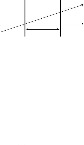
In Fig. 2.11, a geometry is shown which illustrates that two di use fluxes inside the tissue can be distinguished: a flux J1 in the direction of the incident radiation and a backscattered flux J2 in the opposite direction. Two Kubelka–Munk coe cients, AKM and SKM, are defined for the absorption and scattering of di use radiation, respectively4. With these parameters, two di erential equations can be formed:

	dJ1	= −SKMJ1 −AKMJ1 + SKMJ2 ,	(2.39)
	dz
	dJ2	= −SKMJ2 −AKMJ2 + SKMJ1 ,	(2.40)
	dz

where z denotes the mean direction of incident radiation. Each of these equations states that radiance in either direction encounters two losses due to absorption and scattering and one gain due to scattering of photons from the opposite direction. The general solutions to (2.39) and (2.40) can be expressed by

4The coe cients AKM and SKM must be distinguished from α and αs, since the latter are defined for coherent radiation only.

30 2. Light and Matter

J2	AKM	J2	+ d J2
	SKM	SKM
J1		J1	+ d J1
	AKM
θ	z
	d z

Fig. 2.11. Geometry of two fluxes in Kubelka–Munk theory

J1(z) = c11 exp(−γz) + c12 exp(+γz) ,

J2(z) = c21 exp(−γz) + c22 exp(+γz) ,

with

γ = A2KM + 2AKMSKM .

The major problem of Kubelka–Munk theory is the description of AKM and SKM in terms of α and αs. When considering dl as an infinitesimal path length of a scattered photon and dz as an infinitesimal path length of a coherent photon, we may write for the average values

α <dl>= α(b <dz>) = (αb) <dz>= AKM <dz> ,

(2.41)

with some numerical factor b > 1. When also taking the geometry shown in Fig. 2.12 into account, we obtain

		+1
=		−1						,
			+1|			θ	|
<dl>				cos1				J(z) |cosθ| d(cosθ)
<dz>		−1			J(z) |cosθ| d(cosθ)

and, since J does not depend on θ according to our assumption of purely di use scattering,

	<dl>	=	+1 −+11 d(cosθ)	= 2 .	(2.42)
	<dz>
			−1 |cosθ| d(cosθ)

Combining (2.41) and (2.42) leads to

AKM = 2α .

2.5 Photon Transport Theory

31

	/cos	θ
z
d

θ

dz

Fig. 2.12. Path length in a thin layer at scattering angle θ

Because only backscattering is assumed as pointed out in Fig. 2.11, the corresponding relation for SKM is given by

SKM = αs .

The Kubelka–Munk theory is a special case of the so-called many flux theory, where the transport equation is converted into a matrix di erential equation by considering the radiance at many discrete angles. A detailed description of the many flux theory is found in the book by Ishimaru (1978). Beside the two fluxes proposed by Kubelka and Munk, other quantities of fluxes were also considered, as for instance seven fluxes by Yoon et al. (1987) or even twenty-two fluxes by Mudgett and Richards (1971). In general, though, all these many flux theories are restricted to a one-dimensional geometry and to the assumption that the incident light be already di use. Another disadvantage is the necessity of extensive computer calculations.

Di usion Approximation. For albedos a >> 0.5, i.e. if scattering overwhelms absorption, the di use part of (2.37) tends to be almost isotropic. According to Ishimaru (1989), we may then expand the di use radiance Jd in a series by

Jd =	1	(Id + 3Fds + ···) ,	(2.43)
	4π

where Id is the di use intensity, and the vector flux Fd is determined by

Fd(r) = Jd(r,s)s dω .

4π

The first two terms of the expansion expressed by (2.43) constitute the diffusion approximation. The di use intensity Id itself satisfies the following di usion equation

( 2 −κ2)Id(r) = −Q(r) ,

(2.44)

where κ2 is the di usion parameter, and Q represents the source of scattered photons. It was shown by Ishimaru (1978) that

32 2. Light and Matter

κ2 = 3α[α + αs (1 −g)] ,

Q = 3αs(αt + gα)F0 exp(−d) ,

with the incident flux amplitude F0 and the optical depth d as determined by (2.33). According to our previous definition of reduced coe cients in (2.34) and (2.35), we thus have

κ2 = 3ααt .

The di usion equation (2.44) suggests the introduction of an e ective di u- sion length Le and an e ective attenuation coe cient αe of di use light which can be defined by

	Le =		1		=		√	1		,
			κ					3ααt
		1
	αe =					=			3ααt		.
		Le

In general, the di usion approximation thus states that

I = Ic + Id = A exp(−αtz) + B exp(−αe z) ,

(2.45)

with A + B = I0. There exist di erent sets of values for α, αs, and g which provide similar radiances in di usion approximation calculations. They can be expressed in terms of each other by so-called similarity relations given by

α˜ = α ,

α˜s (1 −g˜) = αs (1 − g) ,

where tildes indicate transformed parameters. One motive for applying similarity relations is the transformation of anisotropic scattering into isotropic scattering by using

g˜ = 0 ,

α˜ = α ,

α˜s = αs (1 −g) = αs .

By this transformation, computer calculations are significantly facilitated, since only absorption coe cient and reduced scattering coe cients are needed for the characterization of optical tissue properties.

In Fig. 2.13, the dependence of the di use radiance on optical depth is illustrated in the case of isotropic scattering (g = 0) and di erent albedos (0 < a < 1). For a = 0, attenuation follows Lambert’s law of absorption. For a = 1, the radiance obviously approaches an asymptotic value. It is also interesting to note that just beneath the surface of the scattering medium the di use intensity exceeds the incident intensity, since backscattered photons from deeper layers must be added to the incident intensity.

2.5 Photon Transport Theory

33

Fig. 2.13. Di use intensity as a function of optical depth, assuming the validity of the di usion approximation and isotropic scattering. The ordinate expresses di use intensity in units of incident intensity. Data according to van Gemert et al. (1990)

Monte Carlo Simulations. A numerical approach to the transport equation (2.36) is based on Monte Carlo simulations. The Monte Carlo method essentially runs a computer simulation of the random walk of a number N

of photons. It is thus a statistical approach. Since the accuracy of results

√

based on statistics is proportional to N, a large number of photons has to be taken into account to yield a valuable approximation. Therefore, the whole procedure is rather time-consuming and can be e ciently performed only on large computers. The Monte Carlo method was first proposed by Metropolis and Ulam (1949). It has meanwhile advanced to a powerful tool in many disciplines. Here, we will first point out the basic idea and then briefly discuss each step of the simulation.

The principal idea of Monte Carlo simulations applied to absorption and scattering phenomena is to follow the optical path of a photon through the turbid medium. The distance between two collisions is selected from a logarithmic distribution, using a random number generated by the computer. Absorption is accounted for by implementing a weight to each photon and permanently reducing this weight during propagation. If scattering is to occur, a new direction of propagation is chosen according to a given phase function and another random number. The whole procedure continues until the photon escapes from the considered volume or its weight reaches a given cuto value. According to Meier et al. (1978) and Groenhuis et al. (1983), Monte Carlo simulations of absorption and scattering consist of five principal

34 2. Light and Matter

steps: source photon generation, pathway generation, absorption, elimination, and detection.

–1. Source photon generation. Photons are generated at a surface of the considered medium. Their spatial and angular distribution can be fitted to a given light source, e.g. a Gaussian beam.

–2. Pathway generation. After generating a photon, the distance to the first collision is determined. Absorbing and scattering particles in the turbid medium are supposed to be randomly distributed. Thus, the mean free

path is 1/ σs, where is the density of particles and σs is their scattering cross-section5. A random number 0 < ξ1 < 1 is generated by the computer, and the distance L(ξ1) to the next collision is calculated from

L(ξ1) = − lnξ1 .σs

Since

1

lnξ1 dξ1 = −1 ,

0

the average value of L(ξ1) is indeed 1/ σs. Hence, a scattering point has been obtained. The scattering angle is determined by a second random number ξ2 in accordance with a certain phase function, e.g. the Henyey– Greenstein function. The corresponding azimuth angle Φ is chosen as

Φ = 2π ξ3 ,

where ξ3 is a third random number between 0 and 1.

–3. Absorption. To account for absorption, a weight is attributed to each photon. When entering the turbid medium, the weight of the photon is unity. Due to absorption – in a more accurate program also due to reflection – the weight is reduced by exp[−αL(ξ1)], where α is the absorption coe cient. As an alternative to implementing a weight, a fourth random number ξ4 between 0 and 1 can be drawn. Then, instead of assuming only scattering events in Step 2, scattering takes place if ξ4 < a, where a is the albedo. For ξ4 > a, on the other hand, the photon is absorbed which then is equivalent to Step 4.

–4. Elimination. This step only applies if a weight has been attributed to each photon (see Step 3.). When this weight reaches a certain cuto value, the photon is eliminated. Then, a new photon is launched, and the program proceeds with Step 1.

–5. Detection. After having repeated Steps 1–4 for a su cient number of photons, a map of pathways is calculated and stored in the computer. Thus, statistical statements can be made about the fraction of incident photons being absorbed by the medium as well as the spatial and angular distribution of photons having escaped from it.

5 Absorption will be taken into account by Step 3.

2.5 Photon Transport Theory

35

It has already been mentioned that the accuracy of Monte Carlo simulations increases with the larger numbers of photons to be considered. Due to the necessity of extensive computer calculations, though, this is a very time-consuming process. Recently, a novel approach has been introduced by Graa et al. (1993a) in what they called condensed Monte Carlo simulations. The results of earlier calculations can be stored and used again if needed for the same phase function but for di erent values of the absorption coe cient and the albedo. When applying this alternative technique, a considerable amount of computing time can be saved.

Inverse Adding–Doubling Method. Another numerical approach to the transport equation is called inverse adding–doubling which was recently introduced by Prahl et al. (1993). The term “inverse” implies a reversal of the usual process of calculating reflectance and transmittance from optical properties. The term “adding–doubling” refers to earlier techniques established by van de Hulst (1962) and Plass et al. (1973). The doubling method assumes that reflection and transmission of light incident at a certain angle is known for one layer of a tissue slab. The same properties for a layer twice as thick is found by dividing it into two equal slabs and adding the reflection and transmission contributions from either slab. Thus, reflection and transmission for an arbitrary slab of tissue can be calculated by starting with a thin slab with known properties, e.g. as obtained by absorption and single scattering measurements, and doubling it until the desired thickness is achieved. The adding method extends the doubling method to dissimilar slabs of tissue. With this supplement, layered tissues with di erent optical properties can be simulated, as well.

So far, we have always assumed that the radiance J is a scalar and polarization e ects are negligible. In the 1980s, several extensive studies were done on transport theory pointing out the importance of additional polarizing effects. A good summary is given in the paper by Ishimaru and Yeh (1984). Herein, the radiance is replaced by a four-dimensional Stokes vector, and the phase function by a 4 × 4 M¨uller matrix. The Stokes vector accounts for all states of polarization. The M¨uller matrix describes the probability of a photon to be scattered into a certain direction at a given polarization. The transport equation then becomes a matrix integro-di erential equation and is called a vector transport equation.

In this section, we have discussed di erent methods for solving the transport equation. Among them, the most important are the Kubelka–Munk theory, the di usion approximation, and Monte Carlo simulations. In a short summary, we will now compare either method with each other. The Kubelka– Munk theory can deal with di use radiation only and is limited to those cases where scattering overwhelms absorption. Another disadvantage of the Kubelka–Munk theory is that it can be applied to one-dimensional geometries only. The di usion approximation, on the other hand, is not restricted

36 2. Light and Matter

to di use radiation but is also limited to predominant scattering. In the latter case, though, it can be regarded as a powerful tool. Monte Carlo simulations, finally, provide the most accurate solutions, since a variety of input parameters may be considered in specially developed computer programs. Moreover, two-dimensional and three-dimensional geometries can be evaluated, even though they often require long computation times.

In Fig. 2.14, the intensity distributions inside a turbid medium calculated with either method are compared with each other. Because isotropic scattering is assumed, an analytical solution can also be considered which is labeled “transport theory”. Two di erent albedos, a = 0.9 and a = 0.99, are taken into account. Hence, the coe cient of scattering surpasses the coe - cient of absorption by a factor of 9 or 99, respectively. The accordance of all four approaches is fairly good. The Kubelka–Munk theory usually yields higher values, whereas di usion approximation and Monte Carlo simulation frequently underestimate the intensity.

Fig. 2.14. Comparison of di erent methods for calculating the di use intensity as a function of optical depth. The ordinate expresses di use intensity in units of incident intensity. Isotropic scattering is assumed. Data according to Wilson and Patterson (1986)

2.6 Measurement of Optical Tissue Properties

37

2.6 Measurement of Optical Tissue Properties

In general, there exist several methods for the measurement of optical tissue properties. They focus on di erent quantities such as transmitted, reflected, and scattered intensities. The absorbance itself is di cult to determine, since photons absorbed by the tissue can no longer be used for detection. Therefore, the absorbed intensity is usually obtained when subtracting transmitted, reflected, and scattered intensities from the incident intensity. Depending on the experimental method, either only the total attenuation coe cient or the coe cients of both absorption and scattering can be evaluated. If the angular dependence of the scattered intensity is measured by rotating the corresponding detector, the coe cient of anisotropy can be obtained, as well.

In Fig. 2.15a–c, three commonly used arrangements are illustrated. The simplest setup for measuring total attenuation is shown in Fig. 2.15a. By means of a beamsplitter, typically 50% of the laser radiation is directed on one detector serving as a reference signal. The other 50% is applied to the tissue sample. A second detector behind the sample and on the optical axis of the beam measures the transmitted intensity. By subtracting this intensity from the intensity measured with the reference detector, the attenuation coe cient6 of the tissue can be obtained. The reader is reminded that total attenuation is due to both absorption and scattering. Thus, with this measurement no distinction can be made between these two processes.

In Fig. 2.15b, a setup for the evaluation of the absorbance is shown. Its basic component is called an integrating sphere and was discussed in theoretical studies by Jacquez and Kuppenheim (1955), Miller and Sant (1958), and Goebel (1967). The sphere has a highly reflecting coating. An integrated detector only measures light that has not been absorbed by a sample placed inside the sphere. Usually, the experiment consists of two measurements: one with and the other without the sample. The di erence in both detected intensities is the amount absorbed by the sample. Thus, when taking the geometrical dimensions of the sample into account, its absorption coe cient can be obtained. Frequently, a ba e is positioned between sample and detector to prevent specular reflection from being detected.

A third experiment is illustrated in Fig. 2.15c. Here, the angular dependence of scattering can be measured by moving the detector on a 360◦ rotary stage around the sample. From the detected signals, the corresponding phase function of scattering is obtained. By fitting this result to a given function, e.g. the Henyey–Greenstein phase function, the coe cient of anisotropy can also be evaluated.

6Actually, this method does not lead to the same attenuation coe cient as defined by (2.30), since reflection on the tissue surface should also be taken into account. Specular reflection can be measured by placing a third detector opposite to the beamsplitter. Di use reflection can be evaluated only when using two integrating spheres as will be discussed below.