Ersoy O.K. Diffraction, Fourier optics, and imaging (Wiley, 2006)(ISBN 0471238163)(427s) PEo

298	DIFFRACTIVE OPTICS II

Figure 16.16. The third image used in ODIFIIT investigations.

can be interlaced. However, it was observed experimentally that this interlacing method minimizes the MSE and thus produces the best results. In this scheme, each hologram was divided into 4 4 subholograms. So, the first image, the second image, and the third image were contained in 16 16, 128 128, and 256 256 desired image regions inside the entire image plane, respectively.

Figure 16.17. The reconstruction of the first image from its ODIFIIT hologram.

OPTIMAL DECIMATION-IN-FREQUENCY ITERATIVE INTERLACING TECHNIQUE

299

Figure 16.18. The reconstruction of the second image from its ODIFIIT hologram.

These results showed very accurate reconstructions of the desired images. Compared to the results from the Lohmann method discussed in Section 15.8, there was consequently a significant increase in the reconstruction quality for high resolution gray-scale images.

Like the DOEs designed with the Lohmann method, the transmittance function designed with ODIFIIT can also be coded as ( 1,1) to make binary phase holograms. This can be further extended to code holograms with multiple levels of phase quantization. This corresponds to multilevel phase elements. For example, four levels of phase quantization can be implemented when encoding the hologram.

Figure 16.19. The reconstruction of the third image from its ODIFIIT hologram.

300	DIFFRACTIVE OPTICS II

So at each point in the hologram there would be a phase shift of 0, p=2, p, or 3p=2. This generates a reconstruction with lower MSE because the hologram function has a closer approximation to the actual desired phase at each point.

16.6COMBINED LOHMANN-ODIFIIT METHOD

Since the detour-phase method used in the binary Lohmann method cannot code amplitude and phase exactly in practise, there will always be some amount of inherent error in the reconstruction. Therefore, iterative optimization as in the IIT and ODIFIIT methods should be effective in reducing the final reconstruction error. For this reason, Lohmann’s coding scheme was implemented together with the interlacing technique to create a better method for designing DOEs [Kuhl, Ersoy]. The combined method is called the Lohmann-ODIFIIT method, or LM-ODIFIIT method. In this approach, the desired amplitude and phase of each subhologram point is encoded using a Lohmann cell, but the hologram is divided into interlaced subholograms like in ODIFIIT.

It was discussed in Section 15.4 that three approximations are made for simplicity in designing a Lohmann hologram: (a) sinc½cdnðx þ x0Þ& const, (b) sincðyWnmdnÞ 1; and (c) exp½2piðxPnmdxÞ& 1. The effects of these approximations on the reconstructed image depend on several factors.

The sinc function sinc½cdnðx þ x0Þ& creates a drop-off in intensity in the x- direction proportional to the distance from the center of the image plane. Approximation (a) considers this sinc factor to be nearly constant inside the image region. A small aperture size c results in less drop-off in intensity. However, this also reduces the brightness of the image.

The sinc function sincðyWnmdnÞ indicates a drop-off in intensity similar to (a), but in the y-direction. This sinc function acts like a slight decrease in amplitude transmission by the factor sincðyWnmdnÞ.

The phase shift exp½2piðxPnmdxÞ& causes a phase error that varies with x location in the image plane. This phase error depends on x and P, and ranges from zero to p=2M. Ignoring the phase factor exp½2piðxPnmdxÞ& leads to image deteriotation as if there is a phase error due to an improper aperture shift [Lohmann, 1970].

The solution used to account for the sinc roll-off in the x direction is to divide the desired image by sinc½cdnðx þ x0Þ&. The desired image f ðx; yÞ becomes,

f ðx; yÞ sinc½cdnðx þ x0Þ& :

The same thing cannot be done for the y direction because sincðyWnmdnÞ depends on the aperture parameters Wnm which are based on the desired image. In the LMODIFIIT and quantized LM-ODIFIIT, this sin c factor is accounted for as follows: the desired image is first divided by the sin c factor affecting the x direction, and the hologram is designed. Then, the y dependent sin c factors due to all the apertures are calculated and summed to determine the effect on the output image. The desired

COMBINED LOHMANN-ODIFIIT METHOD

301

Figure 16.20. Reconstruction with the LM-ODIFIIT method.

image is next divided by the y dependent sin c factor just as it was for the x dependent factor. Next, the hologram is designed again, the effect on the output due to the new aperture heights is calculated, and the original desired image is divided by this new factor. This process is repeated until the reconstructed image does not change, or a convergence condition is met.

The phase shift exp½2piðxPnmdxÞ& is accounted for by successive iterations while designing the hologram function.

16.6.1Computer Experiments with the Lohmann-ODIFIIT Method

Figure 16.20 shows the computer reconstruction of the binary ‘‘E’’ image of Figure 15.3 from its LM-ODIFIIT hologram [Kuhl, Ersoy]. Figure 16.21 shows the computer reconstruction of the binary ‘‘E’’ image from its LM-ODIFIIT hologram with four levels of quantization. Figure 16.22 shows the computer reconstruction of

Figure 16.21. Reconstruction with the LM-ODIFIIT method with four levels of phase quantization.

302	DIFFRACTIVE OPTICS II

Figure 16.22. Reconstruction with the LM-ODIFIIT method.

the girl image from its LM-ODIFIIT hologram. A comparison between the output of the Lohmann method, the ODIFIIT, and the LM-ODIFIIT for a 16 16 gray-scale image was also performed. The results are shown in Figure 16.23.

The tables to be discussed next are based on the results obtained with the ‘‘binary E’’ image. Table 16.2 shows the mean square error and diffraction efficiency results of the computer experiments. The MSE represents the difference between the desired image and the reconstructed image inside the desired image region, and the diffraction efficiency is a measure of how much of the incident wave in percent is diffracted into the desired image region. The table includes comparative results for the ODIFIIT, the Lohmann method (LM), the Lohmann method using a constant amplitude for each cell (LMCA), ODIFIIT using Lohmann’s coding method (LMODIFIIT), and LM-ODIFIIT with constant cell amplitude (LMCA-ODIFIIT). All

Figure 16.23. (a), Original image, and reconstructions with (b) the Lohmann method, (c) the ODIFIIT,

(d) the LM-ODIFIIT.

COMBINED LOHMANN-ODIFIIT METHOD					303
	Table 16.2. MSE and diffraction efficiency results
	for binary DOEs.
	Method	MSE			Efficiency (%)
	LM	1			1.2
	ODIFIIT	0.33			5.7
	LMCA	2.03		10 31	5.9
	LM-ODIFIIT	5:9			1.2
	LMCA-ODIFIIT	1			2.1

results are for binary amplitude holograms. Values of c ¼ 1=2 and M ¼ 1 in the Lohmann method were used throughout. For comparison purposes, the MSE occurring in the Lohmann method was normalized to one, so all other MSE values are relative to the Lohmann method.

Table 16.3 shows the results of the computer experiments in which the amplitude and phase of each cell took on quantized values, and the ODIFIIT was applied. Each Lohmann cell is divided into N N smaller squares in N-level quantization. Quantization of amplitude and phase is done as discussed in Section 16.6. MSE is still relative to the MSE from the Lohmann method alone.

The experimental results indicate that the ODIFIIT is better than the Lohmann method in terms of both MSE and efficiency. In the constant amplitue Lohmann method, the error in the image region increased, but efficiency was significantly improved. Basically, this means reconstruction of a brighter image with less definition. This result seems reasonable for the following reasons: less information is used in LMCA, which increases the error, but the amplitude values throughout the hologram are greater due to aperture size always being as large as possible, which increases the brightness. The output displays a reconstruction of the desired image which is brighter, but has ‘‘fuzzy’’ edges. Less reconstruction occurs outside the desired image region further confirming the efficiency increase. In fact, the efficiency of LMCA surpassed the efficiency of ODIFIIT, but the significant increase in MSE is a disadvantage.

The results indicate that LM-ODIFIIT produces an output most resembling the desired image (lowest MSE), while its efficiency is the same as the original Lohmann’s method (LM). Simulations show qualitatively, that LM-ODIFIIT

Table 16.3. MSE and diffraction efficiency results as a function of number of quantization levels in LM-ODIFIIT and LMCA-ODIFIIT.

Levels of Quantization ðNÞ	MSE	Efficiency (%)
2	2.33	0.6
2-CA	0.42	1.4
4	0.19	1.1
4-CA	0.93	1.1

304	DIFFRACTIVE OPTICS II

(a)

(b)

Figure 16.24. (a) The gray-scale image from its LM-ODIFIIT hologram, (b) the same image after the approximations are compensated for in the method.

generated an extremely sharp and uniform image inside the image region. The simulated reconstruction of the girl image especially demonstrates the accuracy of the LM-ODIFIIT, and should be compared to the LM and ODIFIIT results of the same image.

The MSE of the LMCA-ODIFIIT is equal to the MSE of the LM, greater than the MSE of the LM-ODIFIIT, and less than the MSE of the LMCA. Incorporating ODIFIIT into LMCA reduces the error, just as it did for LM. However, considering the extremely small MSE of LM-ODIFIIT, it is somewhat surprising that the MSE of the LMCA-ODIFIIT is not less. As expected, the efficiency of the LMCA-ODIFIIT is greater than the efficiency of the LM-ODIFIIT.

Quantized LM-ODIFIIT with N ¼ 2 had the largest MSE and the lowest efficiency of all the methods. By using so few quantization levels, not enough information remains after encoding to allow for good reconstruction. Anytime the normalized amplitude is less than 1/2, the amplitude is quantized to zero, and phase information is lost. This explains high error and very poor efficiency. By

COMBINED LOHMANN-ODIFIIT METHOD

305

implementing the constant amplitude technique, more phase information is retained. This results in better MSE and efficiency.

For N ¼ 4, MSE dropped significantly, creating a very good reconstruction of the desired image. This method produced a low MSE, second only to the extremely low value of the original LM-ODIFIIT. Also, its efficiency is comparable to all other methods except ODIFIIT and LMCA. Making the amplitude a constant maintains the efficiency, but increases the error.

Figure 16.23 shows that the 128 128 LM and LM-ODIFIIT images display periodic arrays of dots. The horizontal array in the LM image occurs because of the periodic nature of the hologram. This is due to all the cells being symmetric relative to the direction in which the aperture height is adjusted. The horizontal array in the LM-ODIFIIT image occurs for the same reason. However, in the LM-ODIFIIT hologram, it was observed that the phase at each point of the subholograms converged to the same value. This was observed for every subhologram except the first. This gives a periodic nature to the other direction of the hologram, which results in the vertical array of dots.

Up to now, all simulations neglected the sin c roll-off that actually occurs in the physical reconstruction from a binary CGH. The compensating methods discussed in Section 16.7 were further used in simulations to correct for these errors. The computer reconstructions showed excellent homogeneity in the x direction indicating that the x dependent sin c factor was accurately accounted for. Slight variations were present in the y direction, but can be reduced to a desired level by continued iterations. Figure 16.24 shows the computer reconstruction of the gray-scale image E before and after the sin c roll-off corrections were factored into the output.

17

Computerized Imaging Techniques I:

Synthetic Aperture Radar

17.1INTRODUCTION

A number of modern imaging techniques rely on the Fourier transform and related computer algorithms for image reconstruction. For example, synthetic aperture radar (SAR), image reconstruction from projections, including computerized tomography, magnetic resonance imaging (MRI), and confocal microscopy discussed in Chapter 5 are among such techniques.

In this chapter, the SAR principles are discussed. The first SAR image was produced at the University of Michigan in 1958 with a coherent optical processing method since SAR is essentially similar to holography [Cutrona]. In the early 1970s digital signal processing methods were started to be utilized to computerize SAR image processing [Bennett], [Ulaby]. Currently, computerized SAR image processing is what is used in practice.

This chapter consists of ten sections. Section 17.2 describes SAR in general terms. Section 17.3 is on range resolution. In order to achieve high resolution of imaging, it is also necessary to carefully choose the pulse waveform used. This topic is introduced in Section 17.4. Matched filtering discussed in Section 17.5 is used both for maximizing signal-to-noise ratio (SNR) and achieving very sharp pulses. The way sharp pulses with sufficient energy are achieved with matched filtering is discussed in Section 17.6. Section 17.7 is on cross-range resolution.

The topics discussed so far lay the groundwork for SAR imaging. A simplified theory of SAR imaging is discussed in Section 17.8. Image reconstruction with the Fresnel approximation is highlighted in Section 17.9. Another digital SAR image reconstruction algorithm is discussed in Section 17.10.

17.2SYNTHETIC APERTURE RADAR

The word radar is an acronym for RAdio Detection And Ranging, where the letters used are capitalized. Synthetic aperture radar is a technique to create

Diffraction, Fourier Optics and Imaging, by Okan K. Ersoy

Copyright # 2007 John Wiley & Sons, Inc.

306

SYNTHETIC APERTURE RADAR

307

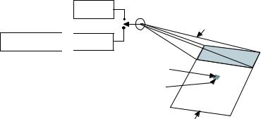
Transmitter

Antenna

Antenna beam

Data processing Receiver

Range resolution

Azimuth resolution

Range interval

Figure 17.1. A visualization of a SAR system.

high-resolution images, which are useful in many areas such as geography, topographic and thematic mapping, oceanography, forestry, agriculture, urban planning, environmental sciences, prediction, and evaluation of natural disasters.

SAR is a coherent imaging technique which makes use of the motion of a radar system mounted on a vehicle such as an aircraft (airborne SAR) or a satellite (spaceborne SAR). A target area is illuminated with the radar’s radiation pattern, resulting in a collection of echoed signals while the vehicle is in motion. These echoed signals are integrated together, using special algorithms, yielding a high-resolution image of the target area.

A simple block diagram for SAR imaging is shown in Figure 17.1. An EM pulse at a microwave frequency is sent by the transmitter and received by the receiver after it gets reflected by the target area. In order to synthesize a large artificial antenna, the flight path in a straight direction is used. In this way, the effective antenna length can be several kilometers. Azimuth (or cross-range) is the direction along the flight path. Range (or slant range) is the direction perpendicular to the azimuth.

One return or echo of the pulse generates information to be used to obtain the image of the target area. High resolution (small pixel sizes) and large signal- to-noise ratio are obtained by illuminating the target area many times with periodically emitted pulses. This is equivalent to signals, each of which is emitted from a single element of a large antenna array. Hence, the name synthetic aperture radar.

The azimuth resolution at range R from an antenna of dimension L is approximately lR=L as shown in Section 17.7. Without the synthetic aperture, making L large at microwave frequencies is impractical. The synthetic aperture corresponds to an antenna array with antenna elements distributed over the flight path.

SAR imaging is often carried out with a satellite system. For example, the Seasat satellite system put into orbit by JPL/NASA in June 1978 had the task of creating SAR images of large regions of the earth’s surface. The Shuttle Imaging Radar (SIR)