Ersoy O.K. Diffraction, Fourier optics, and imaging (Wiley, 2006)(ISBN 0471238163)(427s) PEo

12

Wave Propagation in Inhomogeneous Media

12.1INTRODUCTION

In previous chapters, the index of refraction nðx; y; zÞ was assumed to be constant, independent of position. In many applications, such as wave propagation in optical fibers, volume diffraction gratings, photorefractive media, and so on, nðx; y; zÞ is actually not constant. Then, analysis becomes much more difficult, and often numerical methods are used to analyze wave propagation in such media. Some methods used are pseudospectral, such as the beam propagation method (BPM) discussed in Sections 12.4 and 12.5, whereas others are usually based on finite difference or finite element methods.

The BPM method discussed in this chapter is based on the paraxial wave equation for inhomogeneous media, is valid for propagation near the z-axis, and has several other restrictions. Its main advantage is that it is computed fast with the FFT and is sufficiently accurate in a large number of applications. For wide-angle propagation, other BPM algorithms exist, and they are usually based on the finite difference method. This is further discussed in Chapter 19 in the context of dense wavelength division multiplexing/demultiplexing for optical communications and networking.

This chapter consists of five sections. Section 12.2 discusses the Helmholtz equation for inhomogeneous media. The paraxial wave equation for homogeneous media discussed in Section 5.4 is generalized to inhomogeneous media in Section 12.3. The BPM as a prominent numerical method employing the FFT for wave propagation in inhomogeneous media is introduced in Section 12.4. A particular example of how the BPM is used in practice is the directional coupler illustrated in Section 12.5. This is an optical device consisting of two dielectric wave guides placed nearby so that an optical wave launched into one guide can be coupled into the other. Such devices are of common use in optical communications and networking. It is shown that the BPM gives results sufficiently accurate as compared with the rigorous coupled mode theory. As the coupled mode theory cannot be utilized in more complex designs, the BPM is usually the method of choice in the analysis and synthesis of such devices involving wave propagation in inhomogeneous media.

Diffraction, Fourier Optics and Imaging, by Okan K. Ersoy

Copyright # 2007 John Wiley & Sons, Inc.

188

PARAXIAL WAVE EQUATION FOR INHOMOGENEOUS MEDIA

189

12.2HELMHOLTZ EQUATION FOR INHOMOGENEOUS MEDIA

The Helmholtz equation for homogeneous media in which the index of refraction is constant was derived in Section 4.2. In this section, this is extended to inhomogeneous media. Let uðx; y; z; tÞ represents the wave field at position ðx; y; zÞ and at time t in a medium with the refractive index nðx; y; zÞ with the wavelength l and angular frequency o. According to Maxwell’s equations, it must satisfy the scalar wave equation

r2uðx; y; z; tÞ þ n2ðx; y; zÞk2uðx; y; z; tÞ ¼ 0

ð12:2-1Þ

where k ¼ o=c ¼ 2p=l.

A general solution to the scalar wave equation can be written in the form of

uðx; y; z; tÞ ¼ Uðx; y; zÞ cosðot þ ðx; y; zÞÞ

ð12:2-2Þ

where Uðx; y; zÞ is the amplitude and ðx; y; zÞ is the phase at position ðx; y; zÞ. In complex notation, Eq. (12.2-2) is written as

uðx; y; z; tÞ ¼ Re½Uðx; y; zÞ expð jotÞ&

ð12:2-3Þ

where Uðx; y; zÞ is the complex amplitude equal to jUðx; y; zÞj expð j ðx; y; zÞÞ. Substituting uðx; y; z; tÞ from Eq. (12.2-3) into the wave equation (12.2-1) yields

the Helmholtz equation in inhomogeneous media:

ðr2 þ k2ðx; y; zÞÞUðx; y; zÞ ¼ 0

ð12:2-4Þ

where the position-dependent wave number kðx; y; zÞ is given by

kðx; y; zÞ ¼ nðx; y; zÞk0

ð12:2-5Þ

12.3 PARAXIAL WAVE EQUATION FOR INHOMOGENEOUS MEDIA

The paraxial wave equation for homogenous media was discussed in Section 5.4. In this section, it is extended to inhomogeneous media. Suppose that the variation of index of refraction is given by

nðx; y; zÞ ¼ n þ nðx; y; zÞ

ð12:3-1Þ

where n is the average index of refraction. The Helmholtz equation (12.2-4) becomes

½r2 þ n2k02 þ 2n nk02&U ¼ 0

ð12:3-2Þ

where ð nÞ2k2 term has been neglected.

190 WAVE PROPAGATION IN INHOMOGENEOUS MEDIA

If the field is assumed to be propagating mainly along the z-direction, it can be expressed as

Uðx; y; zÞ ¼ U0		ð12:3-3Þ
	ðx; y; zÞe jkz

0ð Þ where U x; y; z is assumed to be a slowly varying function of z, and k equals nk0.

Substituting Eq. (12.3-3) in the Helmholtz equation yields

r

2U0

þ

2jk

d

U0

þ ð

k2

k2

Þ

U0

¼

0

ð

12:3-4

Þ

dz

As U0ðx; y; zÞ is a slowly varying function of z, Eq. (12.3-3) can be approximated as

d			j		2U	0		2U	0
	U0	¼			d		þ	d		þ ðk2 k2ÞU0	ð12:3-5Þ
dz			2k		dx2			dy2

Equation (12.3-5) is the paraxial wave equation for inhomogeneous media. Equation (12.3-3) allows rapid phase variation with respect to the z-variable to be

factored out. Then, the slowly varying field in the z-direction can be numerically represented along z that can be much coarser than the wavelength for many problems. The elimination of the second derivative term in z in Eq. (12.3-5) also reduces the problem from a second order boundary value problem requiring iteration or eigenvalue analysis, to a first order initial value problem that can be solved by simple ‘‘integration’’ along the z-direction. This also means a time reduction of computation by a factor of at least the number of longitudinal grid points.

The disadvantages of this approach are limiting consideration to fields that propagate primarily along the z-axis (i.e., paraxiality) and also placing restrictions on the index variation, especially the rate of change of index with z. The elimination of the second derivative with respect to z also eliminates the possibility for backward traveling wave solutions. This means devices for which reflection is significant cannot be sufficiently modeled.

12.4BEAM PROPAGATION METHOD

The beam propagation method is a numerical method for approximately simulating optical wave propagation in inhomogeneous media. There are a number of different versions of the BPM method. The one discussed in this section has the constraints that reflected waves can be neglected and all refractive index differences are small [Marcuse].

The BPM can be derived by starting with the angular spectrum method (ASM) discussed in Section 4.3, which is for constant index of refraction, say, n. The BPM

BEAM PROPAGATION METHOD

191

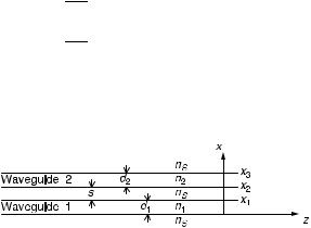
Figure 12.1. Modeling of the inhomogeneous medium for implementing BPM.

can be conceived as a model consisting of homogeneous sections terminated by virtual lenses as shown in Figure 12.1.

The BPM is derived by assuming that the wave is governed in small sections of width z by diffraction as in a homogeneous medium of index n, but with different amounts of phase shift between the sections generated by virtual lenses, modeling the refractive index inhomogeneity. The additional phase shift can be considered to be due to ½nðx; y; zÞ n&. By allowing z to be small, two steps are generated: (1) Wave propagation in a homogeneous medium of index n, which is the average index in the current section, computed with the ASM and (2) the virtual lens effect, which is discussed below.

The effectiveness of this method depends on the choice of z at each step to be small enough to achieve the desired degree of accuracy within a reasonable amount of time.

12.4.1Wave Propagation in Homogeneous Medium with Index n

In each section, the medium is initially assumed to be homogeneous with index of

refraction n.Then, k also equals k. The wave propagation in such a section, say, with
input assumed to be at z								z is computed by the ASM method of Section 4.3.
initial 2		4p	2		2	2
For k				ðfx þ fy Þ so that the evanescent waves are excluded, Uðx; y; zÞ is
expressed as					ðð	Að fx; fy; z zÞ expðþj			k2 4p2ð fx2 þ fy2ÞzÞ
Uðx; y; zÞ ¼
					1			q
					1
					expð j2pð fxx þ fyyÞÞdfxdfy				ð12:4-1Þ

where Að fx; fy; z zÞ is the initial plane wave spectrum given by Eq. (4.3-2). The whole process can be written as

Uðx; y; zÞ ¼ F 1fFfUðx; y; 0Þg expðjmzÞg

ð12:4-2Þ

192	WAVE PROPAGATION IN INHOMOGENEOUS MEDIA

where F and F 1 indicate forward and inverse Fourier transforms, respectively, and m is given by

q
m ¼ n2k2 4p2ð fx2 þ fy2Þ	ð12:4-3Þ

To separate the rapid z-variations caused by large m, it is rewritten in the equivalent form as follows:

4p2ð fx2 þ fy2Þ

m ¼ k

þ q

2

2

2

2

4p

ð fx þ fy Þ

k

k

Hence, Eq. (12.4-2) becomes

Uðx; y; zÞ

j z

ð

!)

¼ F

(FfUðx; y; z zÞg exp

2

2

2 2

1

4p2

fx2 þ fy2

Þ

þ q

k

k 4p ð fx þ fy Þ

ð12:4-4Þ

ð Þ exp jk z

ð12:4-5Þ

12.4.2The Virtual Lens Effect

This is the process of correcting the phase of the complex amplitude Uðx; y; zÞ at the end of each section with a phase function, which is chosen as

GðzÞ ¼ exp½ jkðx; y; zÞ z&	ð12:4-6Þ
GðzÞ satisfies
ðr2 þ k2ðx; y; zÞÞGðzÞ ¼ 0	ð12:4-7Þ

This choice of GðzÞ yields a remarkably accurate phase change for waves traveling nearly parallel to the z-axis.

As nðx; y; zÞ ¼ n þ nðx; y; zÞ and the contribution of the homogeneous medium,

expð jk zÞ, has already been included in Eq. (12.4-5), the phase correction factor

GðzÞ can be written as

ð12:4-8Þ

GðzÞ ¼ expð j½kðx; y; zÞ k& zÞ

Finally, the wave field at z is expressed as

U x; y; z

F 1

8F U x; y; z

z

exp0

j z

4p2ðfx2 þ fy2Þ

19G z

þ

<

B

ð þ

ÞC=

ð Þ ¼

> f ð

Þg

@

qA

> ð Þ

k

k2

4p2 fx2

fy2

>

ð

>:

Þ

:

;

12 4-9

WAVE PROPAGATION IN A DIRECTIONAL COUPLER

193

In some applications such as in integrated optics, the 2-D BPM is used. This is achieved simply by skipping the y-variable related terms.

It is observed that Eq. (12.4-9) is similar to the ASM equation (12.4-5) except for the phase factor GðzÞ. Hence, it can be implemented fast with the FFT as discussed in Section 4.4.

It can be shown that the approximation involved in deriving Eq. (12.4-9) is equivalent to using the paraxial wave equation (12.3-5) derived in Section 12.3 [Feit and Fleck, 1978].

12.5WAVE PROPAGATION IN A DIRECTIONAL COUPLER

As an example of simulation of wave propagation using the BPM, a directional coupler will be discussed. A directional coupler is an optical device used in optical communications, consisting of two parallel dielectric wave guides placed nearby each other so that an optical wave launched into one guide can be coupled into the other. The directional coupler structure is illustrated in Figure 12.2.

12.5.1A Summary of Coupled Mode Theory

To describe waveforms that travel in a directional coupler, the theory of coupled mode equations is used [Saleh and Teich, 1991]. In this section, a brief summary of this theory is given so that the BPM simulation results can be compared with the analytical results obtained with the coupled mode theory.

The peak amplitude variations along z in wave guide i is defined as aiðzÞ for i ¼ 1, 2. The beam intensities are given by jaij2. The coupled mode equations show the power exchange between the two wave guides due to their proximity. They are given by

@a1 ¼ jC21 expðj bzÞa2ðzÞ

@z

ð12:5-1Þ

@a2 ¼ jC12 expð j bzÞa1ðzÞ

@z

where the coefficients b1 and b2 are the uncoupled propagation constants depending on the refractive index in each guide, and b ¼ b1 b2; C12 and C21 are the

Figure 12.2. The directional coupler structure.

194	WAVE PROPAGATION IN INHOMOGENEOUS MEDIA

coupling coefficients defined as follows:

	1	2	2		k2
				0
C12 ¼		ðn1	n	Þ
	2				b2
	1	2	2		k2
				0
C21 ¼		ðn2	n	Þ
	2				b1

ð

u2ðxÞu1ðxÞdx

guide2

ð

u1ðxÞu2ðxÞdx

guide1

ð12:5-2Þ

ð12:5-3Þ

The general solutions for can be derived as follows [Saleh and Teich, 1991]:

a1ðzÞ ¼

A1

cosðgzÞ j 2gbsinðgzÞ A2

jg sinðgzÞ exp þj

2b z

ð12:5-4Þ

C21

a2ðzÞ ¼

A1

jg sinðgzÞ þ A2

cosðgzÞ þ j 2gbsinðgzÞ exp j

2b z

ð12:5-5Þ

C21

where Ai’s are the initial peak amplitudes in the wave guides, and

2

g2

¼

b

þ C2

ð12:5-6Þ

2

¼ p

ð

12:5-7

Þ

C

C12C21

12.5.2Comparison of Coupled Mode Theory and BPM Computations

To show that the BPM is sufficiently accurate for simulation, the wave intensities in two different directional coupler structures were computed with the BPM and compared with the analytical results obtained from the coupled mode theory [Pojanasomboon, Ersoy, 2001]. According to Eqs. (12.5-4) and (12.5-5), the analytical results for the case of zero initial intensity in wave guide 2 ðA2 ¼ 0Þ can be expressed as

2

ja1ðzÞj2

¼ jA1j2

"cos2

ðgzÞ

b

sin2ðgzÞ#

ð12:5-7Þ

2g

ja2ðzÞj2

¼ jA1j2

"

jC21j

2sin2ðgzÞ#

ð12:5-8Þ

g

where

2

b ¼ b1 b2;

g2

¼

b

þ C2

ð12:5-9Þ

2

ð

¼ p

12:5-10

Þ

C

C12C21

WAVE PROPAGATION IN A DIRECTIONAL COUPLER							195

Figure 12.3. Analytical results for power exchange between synchronous wave guides.

12.5.2.1 Case 1: Synchronous Wave guides. The directional coupler in this case has the same refractive index values in both guides, namely, n1 ¼ n2. Because b1 and b2 depend on the refractive index in the guides, this case yields b1 ¼ b2 or b ¼ 0. The intensities in the wave guides are given by

ja1ðzÞj2	¼ jA1j2 cos2ðgzÞ				ð12:5-6Þ
ja2ðzÞj2	¼ jA1j2		jC21j	2sin2ðgzÞ	ð12:5-7Þ
			g

The parameters used in the simulations were A1 ¼ 1, n1 ¼ n2 ¼ 1:1, d1 ¼ d2 ¼ s ¼ 1. The power exchange determined from the analytical expressions is illustrated in Figure 12.3. According to Eqs. (12.5-6) and (12.5-7), complete power exchange can be achieved at z ¼ p=2g.

In the BPM simulation, power at any z in each wave guide is calculated as

ð

jUðx; zÞj2dx:

guide

The results are shown in Figure 12.4. It is observed that the BPM simulation results with the same parameters yield the same general response as in Figure 12.3.

196	WAVE PROPAGATION IN INHOMOGENEOUS MEDIA

Figure 12.4. The BPM simulation of power exchange in directional coupler with synchronous wave guides.

Figure 12.5. Analytical results for power exchange between nonsynchronous wave guides.

WAVE PROPAGATION IN A DIRECTIONAL COUPLER						197

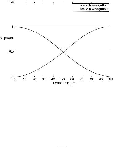
Figure 12.6. BPM simulation of power exchange between nonsynchronous wave guides.

12.5.2.2 Case 2: Nonsynchronous Wave guides. In the nonsynchronous case, the mismatch n1 ¼6 n2 makes b ¼ b1 b2 ¼6 0. The power of the propagating wave in wave guide 2 is obtained as

	"				2sin2ðgzÞ#
ja2ðzÞj2 ¼ jA1j2			jC21j			ð12:5-8Þ
			g

q

The term g ¼ ð b=2Þ2 þ C2 does not allow the quantity in the bracket to be equal to 1. Hence, complete power exchange between the two guides cannot be accomplished at any z as shown in Figure 12.5. The corresponding BPM simulation gives the same results as shown in Figure 12.6.

These results show that the BPM gives highly accurate results as compared with the coupled mode theory in these applications. In more complicated designs such as the nonperiodic grating-assisted directional coupler, the coupled mode theory cannot be used, and the BPM is the method of choice for reliable analysis and subsequent design [Pojanasomboon, Ersoy, 2001].