Ersoy O.K. Diffraction, Fourier optics, and imaging (Wiley, 2006)(ISBN 0471238163)(427s) PEo

218 APODIZATION, SUPERRESOLUTION, AND RECOVERY OF MISSING INFORMATION

the circular aperture has a central lobe whose radius is given by
d ¼	0:61 ld0		ð14:3-1Þ
	R

where d0 is the distance from the circular aperture. d is called the Rayleigh distance and is a measure of the limit by which two point sources can be resolved. Note that d is due to the exit pupil of the optical system, which is a finite aperture.

Finite aperture means the same thing as missing information since the wave field is truncated outside the aperture. Below the wave field is referred to as the signal since the topic discussed is the same as signal recovery in signal processing. In addition, the window function is generalized to be a distortion or transformation operator D, as commonly used in the literature on signal recovery. The coverage will still be in 1-D without loss of generality.

For a space-limited signal, the exact recovery of the signal is theoretically possible since the Fourier transform of such a signal is an analytic function [Stark, 1987]. If an analytic function is exactly known in an arbitrarily small region, the entire function can be found by analytic continuation. Consequently, if only a small part of the spectrum of such a signal is known exactly, the total spectrum and the signal can be recovered.

Unfortunately, especially due to measurement noise, the exact knowledge of part of the spectrum is often impossible. Instead, imperfect measurements and a priori information about the signal, such as positivity, finite extent, etc. are the available information.

The measured signal v can be written in terms of the desired signal u as

v ¼ Du

ð14:3-2Þ

where D is a distortion or transformation operator. With known D, the problem is to recover z (in system identification, the problem is to estimate D when v and u are known).

The straightforward approach to solve for u is to find D 1 such that

u ¼ D 1v v ¼ Du

ð14:3-3Þ

Unfortunately, D is often a difficult transformation. For example, when more than one u corresponds to the same v, D 1 does not exist. Such is the case, for example, when D corresponds to a low-pass filter. Even if D 1 can be approximated, it is often ill-conditioned such that slight errors cause large errors in the estimation of u. The problem of recovery of u under such conditions is often referred to as the inverse problem. In the following sections, signal recovery by contractions and projections will be studied as potential methods for solving inverse problems. These methods are usually implemented in terms of a priori information in the signal and spectral domains.

CONTRACTIONS

219

14.4CONTRACTIONS

In what is discussed below, signals are assumed to be vectors in a complete normed linear vector space. See Appendix B for a discussion of linear vector spaces. Vector norms are discussed in Section B.3. The Euclidian norms to be used below are as follows:

Continuous Signal	2 1					2dt31=2
juj ¼				zðtÞ			ð14:4-1Þ
	4	ð
		1			5
Discrete Signal	"n			ju½n&j2#1=2
juj ¼		1					ð14:4-2Þ
		X
		¼ 1

In the following, the signal u will be assumed to be discrete and to belong to a finite-dimensional vector space S, which can be considered to be a subset of the real space Rn or the complex space Cn, n being the dimension of the space.

Let S0 be a subspace of S. A mapping by an operator A of the vectors in S0 is defined to be nonexpansive if

jAu Avj ju vj

ð14:4-3Þ

for every u and v which belong to S0. The mapping is strictly nonexpansive if inequality holds whenever u 6¼ v.

Linear operators on u are usually represented as matrices. The norm of a matrix can be defined in a number of ways. For example, the spectral norm of the linear operator A is given by

jAj ¼ RðAH AÞ 1=2

ð14:4-4Þ

where AH denotes the complex conjugate transpose of A, and R(B) is the spectral radius of B, which is the largest eigenvalue of B in absolute value. A matrix norm is said to be consistent with a vector norm if

jAuj jAjjxj

ð14:4-5Þ

For example, the spectral norm given by Eq. (14.4-4) is consistent. For a nonexpansive mapping, A must satisfy

jAj 1

ð14:4-6Þ

due to the inequality given by Eq. (14.4-3).

220 APODIZATION, SUPERRESOLUTION, AND RECOVERY OF MISSING INFORMATION

Another topic of importance is the fixed point(s) of the linear operator A. Consider

Au ¼ u

ð14:4-7Þ

Any vector u* which satisfies this equation is called a fixed point of A.

If the mapping A is strictly nonexpansive, and there are two fixed points u* and v*, then

ju v j ¼ jAu Av j < ju v j

ð14:4-8Þ

is a contradiction. It is concluded that there cannot be more than one fixed point in a strictly nonexpansive contraction.

14.4.1Contraction Mapping Theorem

When the mapping by A is strictly nonexpansive so that

jAu Avj ju vj

ð14:4-9Þ

where 0 < a < 1, then, A has a unique fixed point in S0.

Proof:

Let u0 be an arbitrary point in S0. The sequence uk ¼ Auk 1, k ¼ 1; 2; . . . is formed. The sequence ½uk& belongs to S0. We have

jukþ1

ukj ¼ jAuk

Auk 1j ajuk

uk 1j

ð14:4-10Þ

and, by repeated use of Schwarz inequality,

jukþp ukj ¼ jukþp ukþp 1 þ ukþp 1

ukþp 2 þ ukþpþ2 ukj

X

¼

p

ukþi 1j ðap 1 þ ap 2 þ þ 1Þjukþ1

ukj ð14:4-11Þ

jukþi

i¼1

Since

jzkþ1 zkj akjz1

z0j

ð14:4-12Þ

and

a

p 1

þ a

p

2

1

ap

1

ð14:4-13Þ

þ þ 1 ¼

<

;

1 a

1 a

AN ITERATIVE METHOD OF CONTRACTIONS FOR SIGNAL RECOVERY										221
the relation (14.4-11) can be written as
										ð14:4-14Þ
ukþp	uk	1 ak a u1 u0
A sequence [an] is called a Cauchy sequence				if,		given any		2	> 0, there is a positive
integer Nð2Þ such that if n; m > Nð2Þ, it follows that
	jan	amj <2								ð14:4-15Þ

A basic theorem of analysis is that a sequence converges to a fixed point if it is a Cauchy sequence.

The relation (14.4-14) shows that ½uk& is a Cauchy sequence. It follows that

k		Au	k ¼	Au	¼	u	ð	14:4-16	Þ
lim
	!1

where u is the fixed point. In summary, if the mapping by A is strictly nonexpansive, the sequence created by ukþ1 ¼ Auk converges to the unique fixed point u .

14.5 AN ITERATIVE METHOD OF CONTRACTIONS FOR SIGNAL RECOVERY

Assume that there is a measured signal v, which is distorted in some fashion. From v, a more accurate signal is desired to be obtained through iterations. The iterated signal at iteration k is uk, k being an integer for counting iterations. As k increases, uk approaches the recovered signal.

The method to be discussed for this purpose is also known as the method of constrained iterative signal restoration [Schafer]. It is based on the following

iterative equation:
ukþ1 ¼ Fuk	ð14:5-1Þ

where uks are the successive approximations to the recovered signal, and F is an operator. F is obtained both from a distortion operator and a priori knowledge in the form of certain constraints. In general, F is not unique. A simple technique of estimating F is given below.

Prior knowledge can be expressed by a constraint operator:

Cu ! u

ð14:5-2Þ

For example, with a multidimensional signal u, C½u& may be given as

	8 u½n&
Cu½n& ¼	<
	0
	: a

0 u½n& a

u½n& < 0 ð14:5-3Þ u½n& > a

222 APODIZATION, SUPERRESOLUTION, AND RECOVERY OF MISSING INFORMATION

As another example, if u(t) is an analog signal bandlimited by a system to frequencies below fc, Cu(t) can be written as

	1		2 f t
CuðtÞ ¼	ð	uðtÞ	sin p cð	tÞ	dt	ð14:5-4Þ
			pðt tÞ
	1

Every estimate uk of u should be constrained by C. Cuk is interpreted as an approximation to ukþ1. The result Cuk is further processed with a distortion operator D, if any, to yield DCuk. Interpreting DCuk as an estimate of v, the output errorv is defined as

v ¼ v DCuk

ð14:5-5Þ

The recovered signal error between the (k þ 1)th and kth iterations can be defined as

u ¼ ukþ1 Cuk

ð14:5-6Þ

How does u and v relate? The simplest assumption is that they are proportional, say, u ¼ l v. Then,

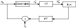
Fuk ¼ ukþ1 ¼ Cuk þ u ¼ Cuk þ lðv DCukÞ

ð14:5-7Þ

This can also be written as

Fuk ¼ lv þ Guk

ð14:5-8Þ

where

G ¼ ðI lDÞC

ð14:5-9Þ

and I is the identity operator. The initial approximation to u can be chosen as u0 ¼ lv.

If F is chosen contractive, uk converges to a fixed-point u . Equation (14.5-8) shows that

jFuk Funj ¼ jGuk Gunj

ð14:5-10Þ

Thus, if F is contractive, so is G. With u0 ¼ lv, Eq. (14.5-8) becomes

Fuk ¼ ukþ1 ¼ u0 þ Guk

ð14:5-11Þ

u00k Þ.

ITERATIVE CONSTRAINED DECONVOLUTION

223

The procedure at the kth iteration according to Eq. (14.5-11) is as follows:

1.Apply the constraint operator C on uk, obtaining u0k.

2.Apply the distortion operator D on u0k, obtaining u00k .

3. Compute ukþ1 as u0 þ lðuk

An example of this method is given below for deconvolution.

14.6ITERATIVE CONSTRAINED DECONVOLUTION

Given v and h, deconvolution involves determining u when v is the convolution of u and h:

v ¼ h u	ð14:6-1Þ
When the iterations start with u0 ¼ lv, Eq. (14.5-8) can be written as
ukþ1 ¼ lv þ ðd lhÞ Cuk	ð14:6-2Þ

where the constraint operator is simply the identity operator for the time being. The FT of Eq. (14.6-2) yields

Ukþ1 ¼ lV þ Uk lHUk

ð14:6-3Þ

where the capital letters indicate the FTs of the corresponding lowercase-lettered variables in Eq. (14.6-2)

Eq. (14.6-3) is a first-order difference equation in the index k. It can be written as

Ukþ1		ð1 lHÞUk ¼ lV					ð14:6-4Þ
whose solution is
		V		lH&kþ1u½k&
Uk ¼			½1				ð14:6-5Þ
		H
where u½k& is the 1-D unit step sequence. As k ! 1, the solution becomes
		U1 ¼			V		ð14:6-6Þ
					H
if
	j1 lHj < 1						ð14:6-7Þ

Equation (14.6-6) is the same result obtained with the inverse filter. The advantage of the interactive procedure is that stopping the iterations after a finite number of steps may yield a better result than the actual inverse filter.

224 APODIZATION, SUPERRESOLUTION, AND RECOVERY OF MISSING INFORMATION

Equation (14.6-7) shows that the procedure will break down if H equals 0 at some frequencies. Equation (14.6-7) can also be written as

Re½H& > 0

ð14:6-8Þ

In order to avoid testing the validity of Eq. (14.6-8) at all frequencies, a better procedure involves convolving both sides of Eq. (14.6-1) with inverted h (h ½ m& in 1-D and h ½ m; n& in 2-D with discrete signals). Then, we get

v0 ¼ x h0

ð14:6-9Þ

where h0 is a new impulse response sequence whose transfer function is given by

H0 ¼ jHj2

ð14:6-10Þ

and v0 is the convolution of v with the inverted h .

In solving Eq. (14.6-9) by the iterative method, Eq. (14.6-8), namely, Re½H0& > 0 is automatically satisfied provided that H 6¼ 0 at any frequency.

Since the iterative solution converges toward the inverse filter solution, it may also end up in an undesirable behavior. For example, a unique result may not be obtained if H ! 0. The use of a constraint operator often circumvents this problem. For example, u may be assumed to be positive over a finite support. In 2-D, the

constraint operator for this purpose is given by

8

uk½m; n& M1 m < M2; N1

n

N2

Cuk m; n

uk m; n 0

14:6-11

½

:

otherwise½ &

ð

Þ

& ¼ <

0

Letting uk0 ¼ Cuk, Eq. (14.6-2) in the DTFT domain becomes

U0

¼ l

V

þ

U0

l

HU0

ð

14:6-12

Þ

kþ1

k

k

The iterations defined by Eq. (14.6-12) can be done by using the DFT. However, u0k ¼ Cuk is to be implemented in the signal domain. The resulting block diagram is shown in Figure 14.4.

Figure 14.4. The block diagram for iterative constrained deconvolution utilizing the Fourier transform.

METHOD OF PROJECTIONS

225

In many applications the impulse response is shift variant. The iterative method discussed above can still be used in the time or space domain, but the algebraic equations in the transform domain are no longer valid.

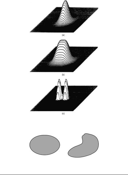
EXAMPLE 14.2 A 2-D Gaussian blurring impulse response sequence is given by

h	m; n	& ¼	exp	m2 þ n2
½				100

The image sequence is assumed to be

u½m; n& ¼ ½dðm 24Þdðn 32Þ þ dðm 34Þdðn 32Þ&

(a)Determine the blurred image v ¼ u h. Visualize h and v.

(b)Compute the deconvolved image with l ¼ 2, 65 iterations, and a positivity constraint.

Solution: (a) The convolution of u and h is given by [Schafer, Mersereau, Richards]

	v m; n		exp	ðm 24Þ2 þ ðn 32Þ2		exp	ðm 34Þ2 þ ðn	32Þ2
		& ¼		100	# þ		100	#
	½		"			"

Plots of h and v are shown in Figure 14.5(a) and (b), respectively.

(b)Figure 14.5(c) shows the deconvolution results after 65 iterations.

14.7METHOD OF PROJECTIONS

A subset of contractions is projections. An operator P is called a projection operator or projector if the mapping Pu satisfies

j

Pu

u

j ¼

v S0

j

v

u

j

ð

14

:

7-1

Þ

inf

2

where u 2 S, and S0 is a subset of S. In the context of signal recovery, S0 is the subset to which the desired signal belongs to. g ¼ Pu is called the projection of u onto S0. This is interpreted as the projection operator P generating a vector g 2 S0 which is closest to u 2 S. G is unique if S0 is a convex set. A very brief review of a convex set is given below.

Let u1 and u2 belong to S0. S0 is convex, if for all l, 0 l 1, lu1 þ ð1 lÞu2 also belongs to S0. A convex set and a nonconvex set are visualized in Figure 14.6.

It can be shown that if S0 is convex, then P is contractive [Youla]. Hence, it is desirable that S0 is indeed convex. If so, the resulting method is called projections onto convex sets. We will consider this case first.

226 APODIZATION, SUPERRESOLUTION, AND RECOVERY OF MISSING INFORMATION

Figure 14.5. Deconvolution of blurred 2-D signal: (a) Gaussian blurring function, (b) blurred signal,

(c) recovered signal by deconvolution [Courtesy of Schafer, Mersereau, Richards].

Convex set

Nonconvex set

Figure 14.6. Examples of a convex set and a nonconvex set.

EXAMPLE 14.3 Consider the set S3 of all real nonnegative functions uðx; yÞ (such as optical field amplitude) that satisfy the energy constraint

ðð

juj2 ¼ juðx; yÞj2dxdy E

Show that S3 is convex.

METHOD OF PROJECTIONS ONTO CONVEX SETS

227

Solution: Consider u1; u2 2 S3. For 0 l 1. The Cauchy–Schwarz inequality to will be used to write

jlu1 þ ð1 lÞu2j lju1j þ ð1 lÞju2j lE1=2

Hence, the set is convex.

EXAMPLE 14.4 Consider the set S4 of all real functions in S whose amplitudes must lie in the closed interval [a,b], a < b, and a 0, b > 0. Show that S4 is convex. Solution: For 0 l 1, we write

u3 ¼ lu1 þ ð1 lÞu2 la þ ð1 lÞa ¼ a

for the lower bound, and

u3 ¼ lu1 þ ð1 lÞu2 lb þ ð1 lÞb ¼ b

for the upper bound. Hence, u3 2 S0, and S4 is convex.

14.8METHOD OF PROJECTIONS ONTO CONVEX SETS

The method of POCS has been successfully used in signal and image recovery. The viewpoint is that every known property of an unknown signal u is considered as a constraint that restricts the signal to be a member of a closed convex set Si. For M properties, there are M such sets. The signal belongs to S0, the intersection of these sets:

\M

S0 ¼ Si	ð14:8-1Þ
i¼1

The signal restoration problem is defined as projecting v, the corrupted version of u, onto S0.

Let Pi denote the projector for the set Si. Let us also define the operator Ti by

Ti ¼ 1 þ liðPi 1Þ

ð14:8-2Þ

If ui is the fixed-point of Pi in Si, we get

T

u

¼

u

þ lið

P

u

u

Þ ¼

u

ð

14:8-3

Þ

i

i

i

i

i

i

i